Boundary modifiers

Boundary modifiers reshape the admissible region before turbines are placed. ExclusionZones removes area, Setback insets the edge and Partition divides the region.

.modify(...) returns a Composite that applies an ordered chain to a copy, so the source boundary is unchanged. The area rule of Boundary shapes applies before modification. Existing turbines are moved by Layout modifiers, and string guides by String modifiers.

import matplotlib.pyplot as plt
import numpy as np
import shapely

import oowl
from oowl import boundaries as B
from oowl import layouts as L
from oowl import modifiers as M
from oowl import strings as S


def show(boundaries, figsize=(12, 3.6)):
    """Plot one row of named boundaries, each titled with its own area."""
    fig, axes = plt.subplots(1, len(boundaries), figsize=figsize)
    for ax, (name, boundary) in zip(axes, boundaries.items()):
        boundary.plot(ax=ax, title=f"{name}\n{boundary.area / 1e6:.1f} km²")
    fig.tight_layout()


def draw_outline(ax, boundary, **style):
    """Trace every ring of a boundary, outer rings and the rims of holes."""
    geometry = boundary.geometry
    polygons = geometry.geoms if geometry.geom_type == "MultiPolygon" else [geometry]
    for polygon in polygons:
        for ring in (polygon.exterior, *polygon.interiors):
            ax.plot(*ring.xy, **style)

Exclusion zones

An exclusion removes a named area such as a wreck, cable corridor or habitat. For a base region \(B\) and exclusions \(E_j\),

\[ B' = B \setminus \bigcup_j E_j . \]

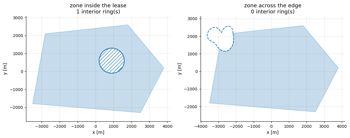
A zone inside \(B\) becomes a hole, and a zone crossing the edge clips the exterior. Any boundary can be a zone. The dashed line is the zone as given.

lease_boundary = B.Polygon(
    [[-3500, -1800], [2500, -2300], [3800, 200], [1800, 2600], [-2800, 2100]]
)
zone = B.Circle(area=np.pi * 700**2, center=(900, 600))
edge_zone = B.SmoothBlob(area=1.5e6, center=(-2800, 1900), roughness=0.3, seed=8)

fig, axes = plt.subplots(1, 2, figsize=(11, 4.4))
excluded = {"zone inside the lease": zone, "zone across the edge": edge_zone}
for ax, (name, shape) in zip(axes, excluded.items()):
    boundary = lease_boundary.modify(M.ExclusionZones([shape]))
    boundary.plot(
        ax=ax, title=f"{name}\n{len(boundary.geometry.interiors)} interior ring(s)"
    )
    draw_outline(ax, shape, ls="--")
fig.tight_layout()

Setbacks

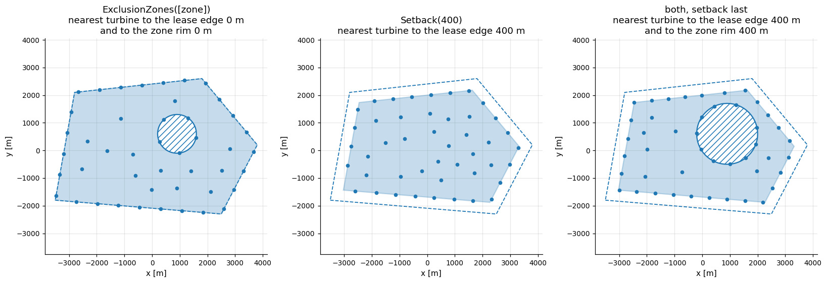
A setback is a margin taken off every edge, including the rims of holes. After an exclusion it therefore widens the hole as well as drawing the outer edge inward. Delaunay places turbines on the boundary, so the nearest turbine measures the clearance the boundary delivers. The dashed line is the original lease.

setback = 400.0
excluded = lease_boundary.modify(M.ExclusionZones([zone]))
boundaries = {
    "ExclusionZones([zone])": (excluded, True),
    f"Setback({setback:.0f})": (lease_boundary.modify(M.Setback(setback)), False),
    "both, setback last": (excluded.modify(M.Setback(setback)), True),
}

fig, axes = plt.subplots(1, 3, figsize=(15, 5.2))
for ax, (name, (boundary, has_zone)) in zip(axes, boundaries.items()):
    farm = oowl.Sampler(boundary, L.Delaunay(45, seed=3)).sample()[0]
    points = shapely.points(farm.positions)
    to_lease = shapely.distance(points, lease_boundary.geometry.boundary).min()
    title = f"{name}\nnearest turbine to the lease edge {to_lease:.0f} m"
    if has_zone:
        to_zone = shapely.distance(points, zone.geometry.boundary).min()
        title += f"\nand to the zone rim {to_zone:.0f} m"
    farm.plot(ax=ax, s=16, title=title)
    draw_outline(ax, lease_boundary, ls="--", lw=1.2)
fig.tight_layout()

The clearance is a minimum. GEOS approximates rounded offsets by chords, so a plain negative buffer erodes slightly less than asked. Setback widens its offset by about 0.12% so the chords lie outside the true arc, and the clearance is always met and exceeded by at most about that, as the delivered margins below show.

shapes = {
    "circle": B.Circle(area=np.pi * 3000**2),
    "convex lease": lease_boundary,
    "lease with a hole": lease_boundary.modify(M.ExclusionZones([zone])),
}
for label, shape in shapes.items():
    for requested in (200.0, 300.0, 500.0):
        inner = shape.modify(M.Setback(requested))
        # The ring-to-ring distance is the narrowest gap the setback opened.
        delivered = shapely.distance(inner.geometry.boundary, shape.geometry.boundary)
        print(
            f"{label:18s} setback {requested:5.0f} m -> {delivered:8.2f} m "
            f"({100 * (delivered - requested) / requested:+.3f} %)"
        )

circle             setback   200 m ->   200.24 m (+0.121 %)
circle             setback   300 m ->   300.36 m (+0.121 %)
circle             setback   500 m ->   500.60 m (+0.121 %)
convex lease       setback   200 m ->   200.24 m (+0.121 %)
convex lease       setback   300 m ->   300.36 m (+0.121 %)
convex lease       setback   500 m ->   500.60 m (+0.121 %)
lease with a hole  setback   200 m ->   200.18 m (+0.090 %)
lease with a hole  setback   300 m ->   300.27 m (+0.090 %)
lease with a hole  setback   500 m ->   500.45 m (+0.090 %)

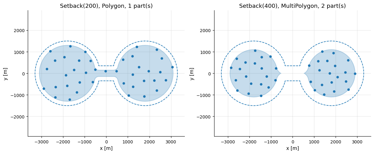
A severed waist is kept, an empty boundary is refused. If a waist is narrower than twice the setback, the boundary splits into a multipolygon and a layout uses both lobes. A setback that consumes the boundary raises ValueError, and so does a negative or non-finite distance.

dumbbell = B.Union(
    [
        B.Circle(area=np.pi * 1500**2, center=(-1800, 0)),
        B.Circle(area=np.pi * 1500**2, center=(1800, 0)),
        B.Rectangle(2.0, 0.30, area=3.24e6, center=(0, 0)),
    ]
)

fig, axes = plt.subplots(1, 2, figsize=(11, 4.6))
for ax, distance in zip(axes, (200.0, 400.0)):
    boundary = dumbbell.modify(M.Setback(distance))
    geometry = boundary.geometry
    n_parts = len(geometry.geoms) if geometry.geom_type == "MultiPolygon" else 1
    farm = oowl.Sampler(boundary, L.PoissonDisc(40, seed=7)).sample()[0]
    farm.plot(
        ax=ax,
        s=18,
        title=f"Setback({distance:.0f}), {geometry.geom_type}, {n_parts} part(s)",
    )
    draw_outline(ax, dumbbell, ls="--", lw=1.2)
fig.tight_layout()

Partitions

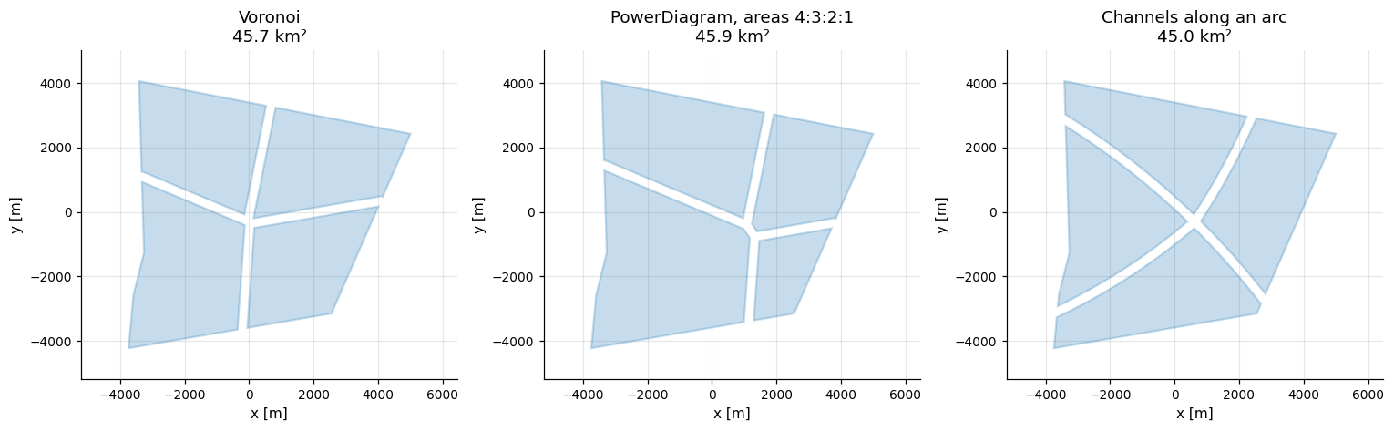
Partition divides a region into n_farms cells kept gap meters apart. Voronoi and PowerDiagram take from each cell the points within half the gap of another, so the cut follows the shared edges and moves smoothly as the boundary is resized. Voronoi gives each site the points nearest it. PowerDiagram fits additive weights \(w_i\) so that the cells

\[ C_i = \{x \mid \lVert x-p_i\rVert^2 - w_i \le \lVert x-p_j\rVert^2 - w_j \text{ for all } j\} \]

of Aurenhammer (1987) match area_weights before the gap is cut. Channels cuts recursively along a string guide, straight by default. Omitted sites are sampled from seed. Composite.parts returns the cells as boundaries, and partition_metadata records the sites, the weight fit or the channel lines. The cells become farms in Multipart boundaries and clusters.

boundary = B.OffshorePolygon(area=50e6, seed=8)
sites = [(-2200, -1200), (-900, 1900), (1600, 1400), (2100, -1500)]
partitioned = {
    "Voronoi": boundary.modify(M.Partition.Voronoi(4, sites=sites, gap=300)),
    "PowerDiagram, areas 4:3:2:1": boundary.modify(
        M.Partition.PowerDiagram(4, area_weights=[4, 3, 2, 1], sites=sites, gap=300)
    ),
    "Channels along an arc": boundary.modify(
        M.Partition.Channels(4, guide=S.Arc(radius=1, span=80), gap=300, seed=2)
    ),
}
show(partitioned, figsize=(14, 4.4))

record = partitioned["PowerDiagram, areas 4:3:2:1"].partition_metadata
print("PowerDiagram area fractions", np.round(record["achieved_area_fractions"], 3))

PowerDiagram area fractions [0.4 0.3 0.2 0.1]

Order of application

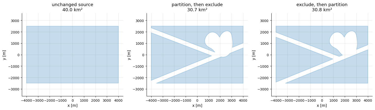
Modifiers apply left to right and do not commute. Partitioning a full rectangle into channel-separated cells differs from partitioning what an exclusion left. Modifying union members before the union can likewise differ from modifying the result.

base = B.Rectangle(8, 5, area=40e6)
exclusion = B.SmoothBlob(area=4e6, center=(2000, 1000), roughness=0.25, seed=8)
orders = {
    "unchanged source": base,
    "partition, then exclude": base.modify(
        M.Partition.Channels(n_farms=3, gap=400, seed=420),
        M.ExclusionZones([exclusion]),
    ),
    "exclude, then partition": base.modify(
        M.ExclusionZones([exclusion]),
        M.Partition.Channels(n_farms=3, gap=400, seed=420),
    ),
}
show(orders, figsize=(14, 4.2))

Resizing a modified boundary

A Sampler given area, a density or a spacing resizes the boundary it draws, see Sampling with a density. A distance given in meters must not scale with it. The base is resized and the chain re-applied, so a setback keeps its distance, a partition keeps its gap and exclusion zones stay where they were given in the plane. The base area is searched so the result has the requested area to rounding, except where a setback or gap makes the area jump as the site grows, and there the nearest size is kept. A chain without such a modifier, like a partition with no gap, scales as a whole together with its cells.

Below, the lease with its zone and setback is sampled at two areas. The hole rim stays the setback away from the fixed zone while the lease around it shrinks.

boundary = lease_boundary.modify(M.ExclusionZones([zone]), M.Setback(setback))
for area in (20e6, 10e6):
    farm = oowl.Sampler(boundary, L.Delaunay(30, seed=3), area=area, seed=1).sample()[0]
    rim = shapely.distance(farm.boundary.geometry.boundary, zone.geometry.boundary)
    print(
        f"{area / 1e6:.0f} km² requested, {farm.boundary.area / 1e6:.6f} km² drawn, "
        f"hole rim {rim:.1f} m from the zone"
    )

20 km² requested, 20.000000 km² drawn, hole rim 400.4 m from the zone
10 km² requested, 10.000000 km² drawn, hole rim 400.4 m from the zone