Describing a population of farms

A Sampler describes a population and is validated as it is built. Any component may be fixed or a specification, meaning a number, a (low, high) range, a frozen scipy.stats distribution, a callable taking one Generator, a Choice, a class, a (constructor, kwargs) recipe, or Literal(value) for data passed through unchanged. Drawing, streaming and replaying a population covers drawing, Sampling with a density sets a density such as the distance between turbines and Concepts explains what a scenario is.

import matplotlib.pyplot as plt
import numpy as np

import oowl
from oowl import boundaries as B
from oowl import layouts as L
from oowl import resources as R
from oowl import sampling as SP
from oowl import strings as S
from oowl import turbines as T

A simple specification

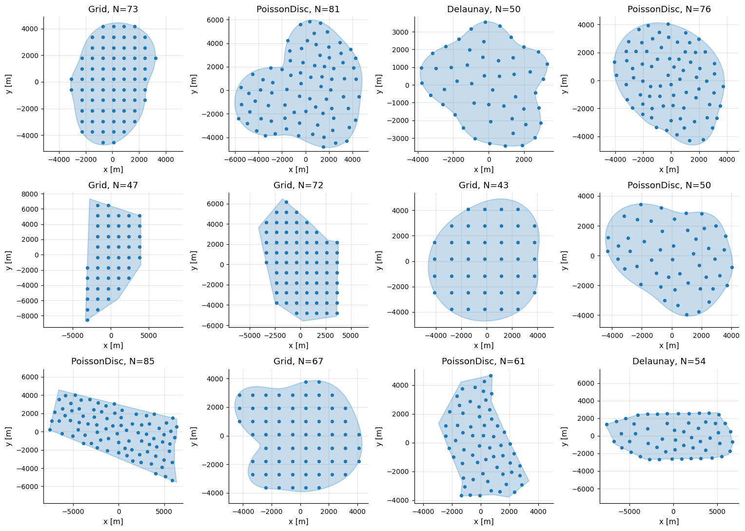
boundary, layout and resource may be positional, and everything else is keyword-only. A class in a Choice is constructed fresh for each scenario with the drawn count and area. A draw returns a tuple of independent scenarios, and each title names the layout family.

simple = oowl.Sampler(
    SP.Choice([B.OffshorePolygon, B.SmoothBlob]),
    SP.Choice([L.Grid, L.PoissonDisc, L.Delaunay]),
    n_turbines=(40, 90),
    area=(30e6, 90e6),
    seed=7,
)

fig, axes = plt.subplots(3, 4, figsize=(14, 10))
for ax, farm in zip(axes.flat, simple.sample(12)):
    family = farm.metadata["sample"]["layout"]["algorithm"]
    farm.plot(ax=ax, s=14, title=f"{family}, N={farm.n_turbines}")
fig.tight_layout()

Nested specifications

A Choice may be nested in another specification, so one boundary choice can serve several branches. Integer pairs are inclusive ranges, pairs containing floats are continuous, and a callable receives its own NumPy generator.

boundary = SP.Choice(
    [
        (B.OffshorePolygon, {"rotation": (0.0, 360.0)}),
        (
            B.SmoothBlob,
            {
                "roughness": (0.05, 0.45),
                "n_harmonics": lambda rng: rng.integers(2, 8),
            },
        ),
        (B.RandomRadialPolygon, {"n_vertices": lambda rng: rng.integers(5, 10)}),
    ],
    probabilities=[0.5, 0.3, 0.2],
)
lattice = SP.Choice(
    [
        (L.Grid, {"rotation": (0.0, 180.0)}),
        (L.Grid, {"lattice_angle": 60, "rotation": (0.0, 180.0)}),
    ]
)
string_layout = (
    L.String,
    {
        "strings": (
            S.Parallel,
            {
                "string": S.Straight,
                "n_strings": lambda rng: rng.integers(3, 8),
                "relative_spacing": (0.1, 0.3),
            },
        ),
    },
)

A recipe head may itself be a Choice. The constructor is chosen first and then given the shared arguments, which every option must accept. A center pair is a point rather than a range, as are the corners, sites and vertices given to exterior, holes, sites and coordinates.

shared_layout = (
    SP.Choice([L.Grid, L.PoissonDisc, L.Sunflower], selection="balanced"),
    {"n_turbines": (25, 45)},
)
chosen = oowl.Sampler(
    boundary=(
        B.Circle,
        {"area": 20e6, "center": (1000.0, 2000.0)},
    ),
    layout=shared_layout,
    seed=12,
).sample(3)
print([farm.metadata["sample"]["layout"]["algorithm"] for farm in chosen])

['Sunflower', 'Grid', 'PoissonDisc']

Values passed through with Literal

A recipe’s constructor may be a function of one’s own, whose arguments the sampler cannot know. A pair given to one of them is a range to draw, so Literal passes it through as it is. A distribution an argument takes itself, rather than one value drawn from it, is wrapped the same way.

def lease(corner, width=4000.0, height=2500.0):
    """A rectangular lease from its south-west corner."""
    x, y = corner
    return B.Polygon([(x, y), (x + width, y), (x + width, y + height), (x, y + height)])


kept = oowl.Sampler(
    (lease, {"corner": SP.Literal((5e5, 6.2e6))}), L.Grid(12), seed=4
).sample()[0]
print("Literal corner:", kept.boundary.geometry.bounds[:2])
try:
    oowl.Sampler((lease, {"corner": (5e5, 6.2e6)}), L.Grid(12), seed=4).sample()
except (TypeError, ValueError) as error:
    print("a plain pair is a range:", error)

Literal corner: (500000.0, 6200000.0)
a plain pair is a range: could not construct lease: cannot unpack non-iterable float object

Correlating components with configuration

configuration overrides boundary, layout, count, area, density, resource, turbines and surface together, a density replacing the sampler’s whole, so a large boundary carries many turbines and a compact one few. A Choice of mappings with selection="balanced" keeps every prefix of the population close to the requested proportions.

configurations = [
    {
        "boundary": boundary,
        "layout": lattice,
        "n_turbines": (70, 120),
        "area": (80e6, 160e6),
    },
    {
        "boundary": boundary,
        "layout": SP.Choice([L.PoissonDisc, L.Delaunay]),
        "n_turbines": (25, 45),
        "area": (18e6, 40e6),
    },
    {
        "boundary": boundary,
        "layout": string_layout,
        "n_turbines": (30, 60),
        "area": (25e6, 60e6),
    },
]
varied = oowl.Sampler(
    configuration=SP.Choice(
        configurations, probabilities=[0.4, 0.4, 0.2], selection="balanced"
    ),
    seed=101,
)
scenarios = varied.sample(8)

fig, axes = plt.subplots(2, 4, figsize=(15, 7.5))
for ax, farm in zip(axes.flat, scenarios):
    family = farm.metadata["sample"]["layout"]["algorithm"]
    farm.plot(ax=ax, s=14, title=f"{family}, N={farm.n_turbines}")
fig.tight_layout()

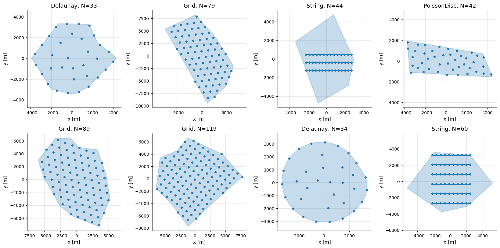
metadata["sample"] holds each farm’s index and resolved components, and summary adds metrics. Count and area tend to rise together.

[
    {
        "index": farm.metadata["sample"]["index"],
        "layout": farm.metadata["sample"]["layout"]["algorithm"],
        **farm.summary(["n_turbines", "region_area"]),
    }
    for farm in scenarios
]

[{'index': 0,
  'layout': 'Delaunay',
  'n_turbines': 33,
  'region_area': 35200151.71515746},
 {'index': 1,
  'layout': 'Grid',
  'n_turbines': 79,
  'region_area': 119592122.97268836},
 {'index': 2,
  'layout': 'String',
  'n_turbines': 44,
  'region_area': 35198420.41582571},
 {'index': 3,
  'layout': 'PoissonDisc',
  'n_turbines': 42,
  'region_area': 19650888.86170616},
 {'index': 4,
  'layout': 'Grid',
  'n_turbines': 89,
  'region_area': 99495734.53156087},
 {'index': 5,
  'layout': 'Grid',
  'n_turbines': 119,
  'region_area': 112665491.76661433},
 {'index': 6,
  'layout': 'Delaunay',
  'n_turbines': 34,
  'region_area': 31314040.181794077},
 {'index': 7,
  'layout': 'String',
  'n_turbines': 60,
  'region_area': 49149061.43379717}]

Linking values with Link

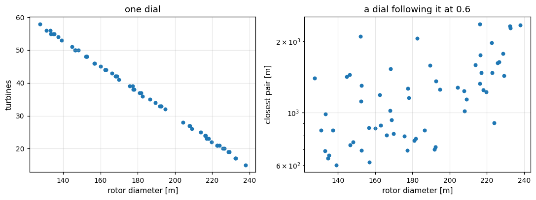
A Link is a dial between 0 and 1 that several values read, so they move together. Here one dial sets the rotor and the count, whose range runs from 60 down to 15, so a larger rotor comes with fewer turbines. A second dial follows the first at a rank correlation of 0.6 and sets the spacing on a log scale. Count and spacing are given, so each area follows.

machine = SP.Link()
spread = SP.Link(follows=machine, correlation=0.6)
turbine = (
    T.Idealized,
    {
        "rated_power": 15e6,
        "rotor_diameter": machine((120.0, 240.0)),
        "hub_height": 150.0,
        "cp_max": 0.46,
    },
)
linked = oowl.Sampler(
    B.OffshorePolygon,
    (L.Grid, {"n_turbines": machine((60, 15))}),
    turbines=turbine,
    density={"minimum_spacing": spread((600.0, 2400.0), scale="log")},
    seed=3,
).sample(60)

rotor = [farm.turbines.rotor_diameter for farm in linked]
fig, axes = plt.subplots(1, 2, figsize=(10, 3.8))
axes[0].scatter(rotor, [farm.n_turbines for farm in linked], s=18)
axes[0].set(xlabel="rotor diameter [m]", ylabel="turbines", title="one dial")
axes[1].scatter(rotor, [farm.minimum_spacing() for farm in linked], s=18)
axes[1].set(
    xlabel="rotor diameter [m]",
    ylabel="closest pair [m]",
    yscale="log",
    title="a dial following it at 0.6",
)
fig.tight_layout()

A linked Choice splits the dial into bands sized by its probabilities, in list order, and linked values inside the chosen recipe read the dial stretched across that band. Link(selection="balanced") spreads the dial evenly over the population, and per="farm" turns it once per farm of a cluster instead of once per scenario. Each scenario records its dials in metadata["sample"]["links"].

Writing your own surroundings

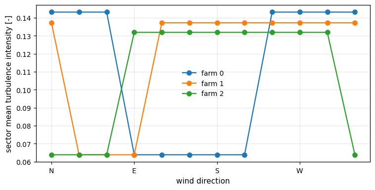
Any value may be a function of the random generator. Here each farm gets a coastline, with offshore sectors over a random arc of 90 to 180 degrees of wind direction and onshore sectors of random roughness elsewhere. Each sector has its own surface, so turbulence differs between the offshore and onshore sectors.

def coastline(rng):
    start, width = rng.uniform(0.0, 360.0), rng.uniform(90.0, 180.0)
    land = float(10 ** rng.uniform(-1.5, -0.5))
    offshore = (30.0 * np.arange(12) - start) % 360.0 < width
    return tuple(R.Charnock() if water else land for water in offshore)


coastal = oowl.Sampler(
    B.OffshorePolygon,
    L.Grid(40),
    resource=(R.WindResource, {"roughness_length": coastline}),
    area=40e6,
    seed=2,
).sample(3)

fig, ax = plt.subplots(figsize=(7.0, 3.6))
for index, farm in enumerate(coastal):
    resource = farm.resource
    ax.plot(
        resource.theta,
        resource.sector_turbulence_intensity,
        marker="o",
        label=f"farm {index}",
    )
ax.set_xticks([0.0, 90.0, 180.0, 270.0], ["N", "E", "S", "W"])
ax.set(xlabel="wind direction", ylabel="sector mean turbulence intensity [-]")
ax.legend(frameon=False)
fig.tight_layout()