Multipart boundaries and clusters

n_farms on the sampler separates one farm in several parts from several farms.

import matplotlib.pyplot as plt
from shapely.geometry import Point

import oowl
from oowl import boundaries as B
from oowl import layouts as L
from oowl import modifiers as M
from oowl import sampling as SP

One farm in several parts

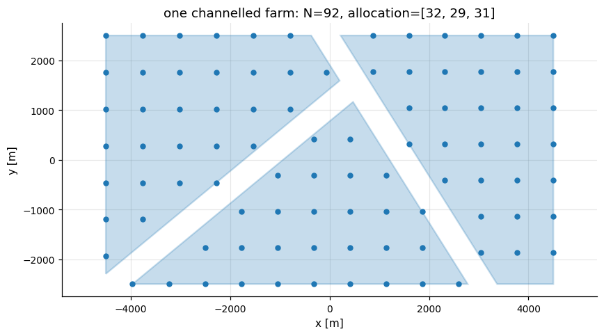
Without n_farms, a divided boundary is one farm with one layout. The count is split deterministically across parts by area and sums to exactly \(N\). Metadata records each slice.

channelled = B.Rectangle(9, 5, area=45_000_000).modify(
    M.Partition.Channels(n_farms=3, gap=500, seed=3)
)
farm = oowl.Sampler(channelled, L.Grid(n_turbines=92, seed=7)).sample()[0]
allocation = [component["n_turbines"] for component in farm.metadata["components"]]

fig, ax = plt.subplots(figsize=(8, 4.5))
farm.plot(
    ax=ax,
    title=f"one channelled farm: N={farm.n_turbines}, allocation={allocation}",
)
fig.tight_layout()

Partition cells as farms

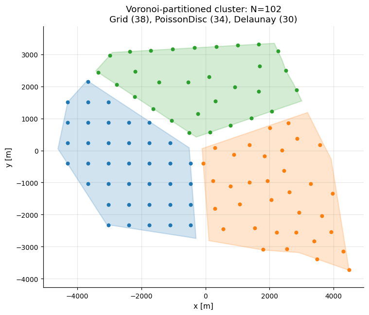
With n_farms=3, a boundary of exactly three parts makes each part a farm with its own layout and exact count. Every multi-farm scenario is a Cluster that saves, loads and summarizes as a whole, and n_farms=1 also returns one. The partition methods are compared in Boundary modifiers.

partitioned = B.OffshorePolygon(area=45_000_000, seed=1).modify(
    M.Partition.Voronoi(
        n_farms=3, sites=[(-2200, -1500), (1800, -1200), (500, 2600)], gap=400
    )
)
cell_layouts = {
    "Grid": L.Grid(38, seed=1),
    "PoissonDisc": L.PoissonDisc(34, seed=2),
    "Delaunay": L.Delaunay(30, seed=3),
}
cluster = oowl.Sampler(partitioned, list(cell_layouts.values()), n_farms=3).sample()[0]

cells = ", ".join(
    f"{name} ({member.n_turbines})" for name, member in zip(cell_layouts, cluster.farms)
)

fig, ax = plt.subplots(figsize=(7, 6))
cluster.plot(
    ax=ax, s=18, title=f"Voronoi-partitioned cluster: N={cluster.n_turbines}\n{cells}"
)
fig.tight_layout()

Saving a cluster

Cluster.save writes each farm as a windIO document, a system with its site where it has a boundary and a layout where it has none, and a manifest.json holding the cluster’s metadata and every farm’s. A resource or surface that several farms share is written once and included. Cluster.load reads them back with their partition cells, so the farms keep their metadata as well as their positions.

import tempfile
from pathlib import Path

with tempfile.TemporaryDirectory() as folder:
    directory = cluster.save(Path(folder) / "cluster")
    print("files:", sorted(path.name for path in directory.iterdir()))
    loaded = oowl.Cluster.load(directory)
kept = [
    (farm.positions == again.positions).all() and farm.metadata == again.metadata
    for farm, again in zip(cluster, loaded)
]
print(f"{loaded.n_farms} farms reloaded, positions and metadata kept: {kept}")

files: ['farm_0000.yaml', 'farm_0001.yaml', 'farm_0002.yaml', 'manifest.json']
3 farms reloaded, positions and metadata kept: [True, True, True]

Neighboring farms

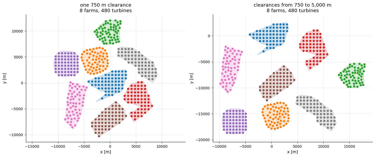
Boundaries without an explicit center are arranged automatically. Positioned ones stay put.

Boundary options are (constructor, {"area": ...}) recipes, built per farm so each farm gets its own shape. A pre-seeded instance in the Choice repeats one shape.

A scalar gap gives a compact cluster with one clearance. A (minimum, maximum) range draws each farm’s clearance from it, so the clearance varies and the minimum stays a hard limit.

boundary_choice = SP.Choice(
    [
        (B.OffshorePolygon, {"area": 24_000_000}),
        (B.SmoothBlob, {"area": 20_000_000, "roughness": 0.12}),
        (B.RandomRadialPolygon, {"area": 18_000_000}),
    ]
)
layout_choice = SP.Choice(
    [L.Grid(60), L.PoissonDisc(60), L.Delaunay(60)],
    probabilities=[0.5, 0.25, 0.25],
)
gaps = {"one 750 m clearance": 750, "clearances from 750 to 5,000 m": (750, 5000)}

fig, axes = plt.subplots(1, 2, figsize=(13, 5.5))
for ax, (label, gap) in zip(axes, gaps.items()):
    neighbors = oowl.Sampler(
        boundary_choice, layout_choice, n_farms=8, gap=gap, seed=7
    ).sample()[0]
    neighbors.plot(
        ax=ax,
        title=f"{label}\n{neighbors.n_farms} farms, {neighbors.n_turbines} turbines",
    )
fig.tight_layout()

Scattering sites across a domain

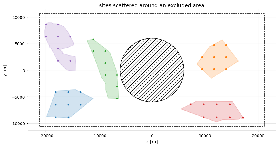
A domain scatters farms within a region, gap meters apart, until n_sites are placed, here all 5. A site that finds no room is replaced by another, and 12 in a row that find none end the fill. An ExclusionZones modifier on the domain excludes whole farms. The layout count is the cluster total, shared across sites. The share of the domain developed is recorded as coverage. Plots draw the domain beneath the farms unless regions=False.

exclusion = Point(0.0, 0.0).buffer(6_000.0)
domain = B.Rectangle(2, 1, area=900_000_000).modify(M.ExclusionZones([exclusion]))
scattered = oowl.Sampler(
    (B.OffshorePolygon, {"area": 30_000_000}),
    L.Grid(40),
    domain=domain,
    n_sites=5,
    gap=2_000.0,
    seed=5,
).sample()[0]

placement = scattered.metadata["placement"]
print(f"{scattered.n_farms} farms carrying {scattered.n_turbines} turbines")
print(f"per farm: {[farm.n_turbines for farm in scattered]}")
print(f"share of the domain developed: {placement['coverage']:.1%}")
print(
    "no site inside the exclusion:",
    not any(farm.boundary.geometry.intersects(exclusion) for farm in scattered),
)

fig, ax = plt.subplots(figsize=(9.0, 4.8))
scattered.plot(ax=ax, s=8, title="sites scattered around an excluded area")
fig.tight_layout()

5 farms carrying 40 turbines
per farm: [8, 8, 8, 8, 8]
share of the domain developed: 19.1%
no site inside the exclusion: True