Spatial metrics

oowl.metrics describes layout geometry, not wake loss, yield or cost. Every metric accepts a Farm or an \((N,2)\) array of positions. Area-based metrics use the boundary area \(A\) of a Farm, or the convex hull of the positions when there is no boundary or boundary=False is passed. The hull is usually smaller than the boundary, so the two are not comparable. The intensity is \(\hat\lambda=N/A\), reported as density in turbines per square meter.

import matplotlib.pyplot as plt
import numpy as np
from matplotlib.collections import PolyCollection

import oowl
from oowl import boundaries as B
from oowl import layouts as L
from oowl import metrics as MET
from oowl import strings as S

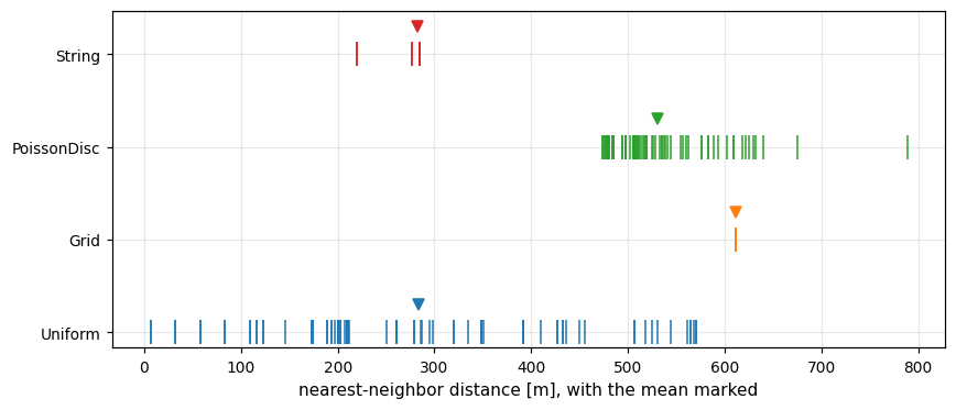
Four families from Layout families share one boundary, turbine count and seed.

n = 80
boundary = B.SmoothBlob(area=np.pi * 3000**2, roughness=0.2, seed=5)
guide = S.Parallel(
    S.Straight(), n_strings=4, relative_spacing=0.14, rotation_spread=5, seed=6
)
families = {
    "Uniform": L.Uniform(n, seed=0),
    "Grid": L.Grid(n, seed=0),
    "PoissonDisc": L.PoissonDisc(n, seed=0),
    "String": L.String(guide, n, seed=0),
}
examples = {
    name: oowl.Sampler(boundary, layout).sample()[0]
    for name, layout in families.items()
}

MET.summary evaluates named entries of MET.SCALAR_METRICS, by default those in MET.DEFAULT_SUMMARY_METRICS. Farm.summary does the same. hull_area measures the turbines’ convex hull and ignores the boundary.

print("defaults:", MET.DEFAULT_SUMMARY_METRICS)
rows = {name: MET.summary(farm, MET.SCALAR_METRICS) for name, farm in examples.items()}
print(f"{'':20s}" + "".join(f"{name:>13s}" for name in examples))
for key in rows["Grid"]:
    print(f"{key:20s}" + "".join(f"{rows[name][key]:13.4g}" for name in examples))

defaults: ('n_turbines', 'nearest_neighbor_mean', 'nearest_neighbor_variation', 'density', 'region_area')

                          Uniform         Grid  PoissonDisc       String
n_turbines                     80           80           80           80
nearest_neighbor_mean        283.9        611.4        530.9        282.9
nearest_neighbor_variation       0.5413    3.126e-16       0.1051      0.03579
density                 2.829e-06    2.829e-06    2.829e-06    2.829e-06
region_area             2.827e+07    2.827e+07    2.827e+07    2.827e+07
clark_evans                0.9549        2.057        1.786       0.9518
aspect_ratio                 1.15        1.011        1.016        1.913
bounding_box_diagonal         7795         7781         8175         6018
quadrat_p_value            0.4848       0.9797    5.412e-06     0.006831
hull_area                 2.3e+07     2.56e+07    2.597e+07    1.226e+07

Nearest-neighbor spacing and Clark-Evans ratio

The nearest-neighbor distance of turbine \(i\) is \(d_i=\min_{j\ne i}\|\mathbf x_i-\mathbf x_j\|\). Its mean \(\bar d\) is nearest_neighbor_mean and its coefficient of variation \(\operatorname{sd}(d_i)/\bar d\) is nearest_neighbor_variation, which is zero for a lattice. Under complete spatial randomness (CSR) the Clark-Evans ratio is

\[ R=\frac{\bar d}{E[d]_{\mathrm{CSR}}}, \qquad E[d]_{\mathrm{CSR}}=\frac12\sqrt{\frac{A}{N}}, \]

with \(R>1\) for dispersion and \(R<1\) for clustering. No edge correction is applied, so \(R\) is descriptive. See Clark and Evans, “Distance to Nearest Neighbor as a Measure of Spatial Relationships in Populations”, Ecology 35 (1954), 445-453.

fig, ax = plt.subplots(figsize=(8, 3.5))
for row, farm in enumerate(examples.values()):
    distances = MET.nearest_neighbor_distances(farm)
    (line,) = ax.plot(distances, np.full(len(distances), row), "|", ms=14)
    ax.plot(MET.nearest_neighbor_mean(farm), row + 0.3, "v", color=line.get_color())
ax.set_yticks(range(len(examples)), list(examples))
ax.set_xlabel("nearest-neighbor distance [m], with the mean marked")
fig.tight_layout()

Ripley’s K and L

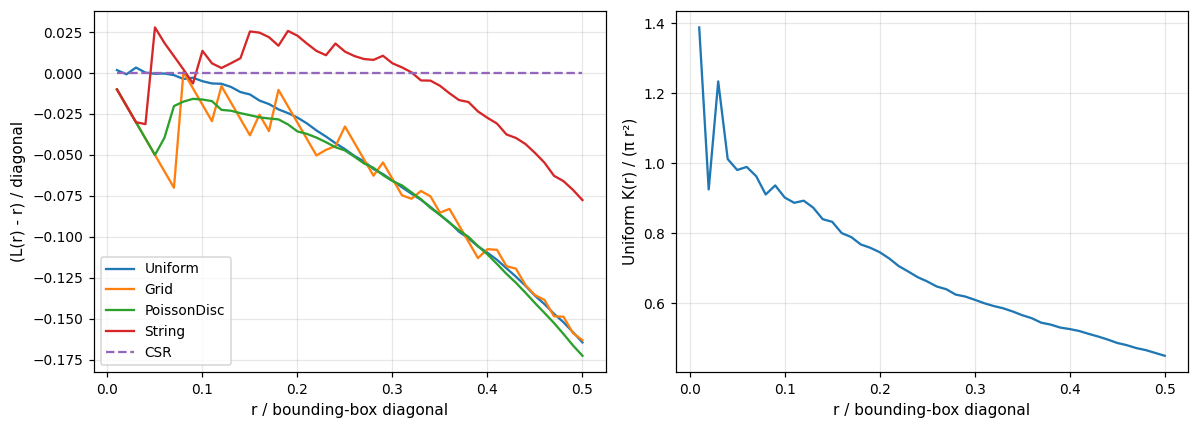
The uncorrected estimator at radius \(r\) is

\[ \hat K(r)=\frac{A}{N^2} \sum_{i\ne j}\mathbf 1\!\left(\|\mathbf x_i-\mathbf x_j\|\le r\right), \qquad L(r)=\sqrt{\hat K(r)/\pi}, \]

with \(K(r)=\pi r^2\) and \(L(r)=r\) under CSR. Positive \(L(r)-r\) means more neighbors than CSR at that scale and negative means regularity. Without edge correction, pairs are lost at large radii, as the CSR Uniform layout shows on the right. See Ripley, “Modelling Spatial Patterns”, Journal of the Royal Statistical Society B 39 (1977), 172-212.

fractions = np.linspace(0.01, 0.5, 50)
fig, (left, right) = plt.subplots(1, 2, figsize=(11, 4))
for name, farm in examples.items():
    diagonal = MET.bounding_box_diagonal(farm)
    curve = MET.ripley_l(farm, fractions * diagonal) / diagonal - fractions
    left.plot(fractions, curve, label=name)
left.plot(fractions, 0 * fractions, "--", label="CSR")
left.set(xlabel="r / bounding-box diagonal", ylabel="(L(r) - r) / diagonal")
left.legend()

radii = fractions * MET.bounding_box_diagonal(examples["Uniform"])
right.plot(fractions, MET.ripley_k(examples["Uniform"], radii) / (np.pi * radii**2))
right.set(xlabel="r / bounding-box diagonal", ylabel="Uniform K(r) / (π r²)")
fig.tight_layout()

Quadrat test

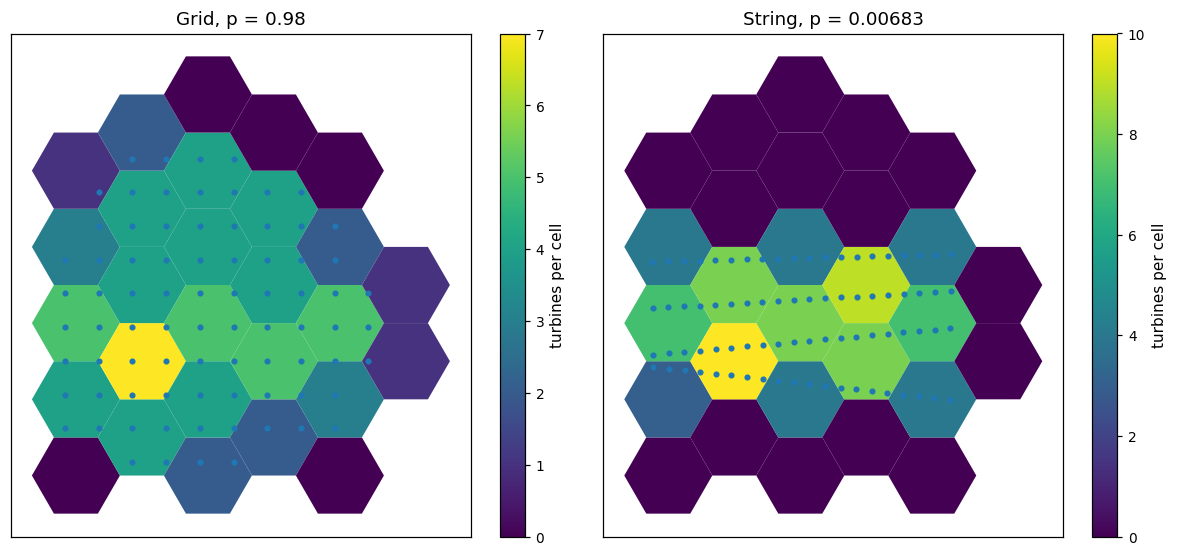
quadrat_window returns the study region, buffered to cover every turbine, and the side \(\ell_h=f\sqrt A\) of a flat-top hexagonal lattice, with \(f\) the hexagon_fraction. hexagon_centers places the cells, hexagon_vertices draws one and quadrat_counts assigns each turbine to its nearest center. With \(a_j\) the area of cell \(j\) inside the region,

\[ E_j=N\,\frac{a_j}{\sum_k a_k}, \qquad X^2=\sum_{j}\frac{(O_j-E_j)^2}{E_j}. \]

quadrat_p_value is the chi-square upper tail of \(X^2\). A low p-value rejects CSR toward clustering. A high one only fails to reject CSR and is not evidence of regularity.

fig, axes = plt.subplots(1, 2, figsize=(11, 5))
for ax, name in zip(axes, ["Grid", "String"]):
    farm = examples[name]
    window, side = MET.quadrat_window(farm)
    centers = MET.hexagon_centers(window, side)
    cells = PolyCollection([MET.hexagon_vertices(x, y, side) for x, y in centers])
    cells.set_array(MET.quadrat_counts(farm, centers))
    ax.add_collection(cells)
    ax.plot(farm.x, farm.y, ".")
    fig.colorbar(cells, ax=ax, label="turbines per cell")
    ax.set(aspect="equal", xticks=[], yticks=[])
    ax.set_title(f"{name}, p = {MET.quadrat_p_value(farm):.3g}")
fig.tight_layout()

Extent and anisotropy

bounding_box_diagonal is the diagonal of the axis-aligned bounds of the positions and depends on orientation. With \(\lambda_1\ge\lambda_2\) the eigenvalues of the position covariance, aspect_ratio is \(\sqrt{\lambda_1/\lambda_2}\), which is 1 for an isotropic layout and grows toward a line. Both appear in the table above.