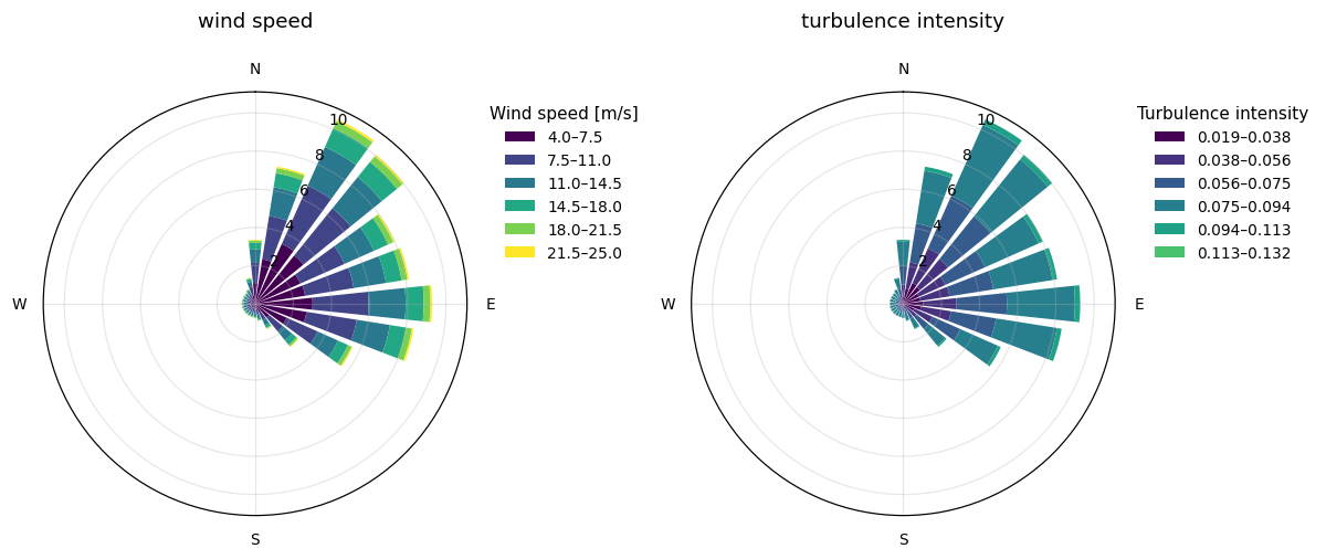
Stability and turbulence

Every case carries the inverse Obukhov length \(1/L\) in \(\mathrm{m}^{-1}\), positive when stable. SiteConditions.stability_parameter(height) returns \(\zeta = z/L\).

The figures here are plain Matplotlib, so oowl.plotting.use_style() gives them the sizes of OOWL’s own plots.

import matplotlib.pyplot as plt
import numpy as np
from scipy import stats

from oowl import resources as R
from oowl.plotting import use_style

use_style()

resource = R.WindResource(mean_wind_speed=9.0)
conditions = resource.sample(4096, seed=1)
zeta = conditions.stability_parameter(resource.reference_height)
print(f"median zeta {np.median(zeta):+.2f}, unstable {np.mean(zeta < 0):.0%}")

median zeta -0.21, unstable 60%

Stability climate

R.KellyGryning draws \(1/L\) from the distribution of Kelly and Gryning (2010),

\[P(L^{-1}) = n_\pm\,\frac{C_\pm}{\sigma_\pm\,\Gamma(5/2)} \exp\!\left[-\left(\frac{C_\pm\,|L^{-1}|}{\sigma_\pm}\right)^{2/3}\right], \qquad \sigma_\pm = \frac{g}{T_0}\,\frac{\operatorname{std}_\pm(H)}{\langle u_*\rangle^3},\]

with \(C_+ = 1\) and \(C_- = 3\). OOWL conditions the scales on each case’s neutral \(u_* = \kappa U / \ln(z/z_0)\) and may tabulate the unstable fraction over it,

\[\sigma_+(u_*) = \sigma_+\left(\frac{\langle u_*\rangle}{u_*}\right)^{p_+}, \qquad \sigma_-(u_*) = \sigma_-\left(\frac{\langle u_*\rangle}{u_*}\right)^{p_-}, \qquad n_-(u_*) \text{ interpolated from a table}.\]

\(p_+ = 2\) keeps \(\theta_*\) and \(p_- = 3\) keeps \(H\) in \(1/L = -\kappa g H/(T_0 u_*^3)\). R.KellyGryning.fit estimates the climate from a record by maximum likelihood, the exponents too with fit_exponents. At Høvsøre it gives \(p_\pm\) of 2.29 and 2.55, with scales within 2 percent of those for 2 and 3. Below, it recovers the unstable fractions and exponents of a synthetic record drawn with \(p_+ = 2\) and \(p_- = 3\).

record_model = R.KellyGryning(
    unstable_fraction=(0.45, 0.28, 0.5),
    stable_scale=0.0068,
    unstable_scale=0.0116,
    fraction_friction_velocity=(0.2, 0.4, 0.6),
)
surface = {"height": 100.0, "roughness_length": 0.017}
rng = np.random.default_rng(0)
speed = rng.uniform(4.0, 25.0, 50_000)
record = record_model.sample(speed, rng.uniform(size=speed.size), **surface)

fitted = R.KellyGryning.fit(
    record, speed, fraction_bins=16, fit_exponents=True, **surface
)
probe = np.array([5.0, 9.0, 16.0])
print(
    "unstable fraction",
    record_model.fractions(probe, **surface).round(2),
    fitted.fractions(probe, **surface).round(2),
)
print("exponents", round(fitted.stable_exponent, 2), round(fitted.unstable_exponent, 2))

unstable fraction [0.42 0.3  0.5 ] [0.43 0.3  0.5 ]
exponents 2.03 3.01

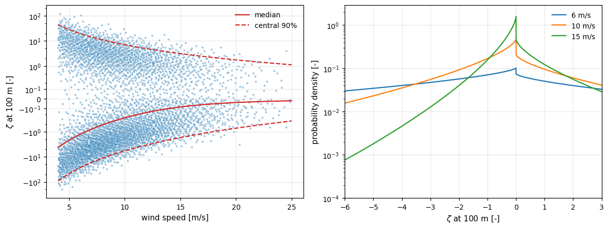
The central 90 percent of \(\zeta\) narrows as the wind rises, and at fixed speed each side follows the 2/3 law.

wind_speed = np.linspace(4.0, 25.0, 160)
surface = {"height": 100.0, "roughness_length": resource.roughness_length}
low, high = resource.stability.bounds(wind_speed, coverage=0.90, **surface)
median = resource.stability.sample(
    wind_speed, np.full(wind_speed.shape, 0.5), **surface
)

fig, axes = plt.subplots(1, 2, figsize=(11.0, 4.2))
axes[0].scatter(conditions.wind_speed, zeta, s=3, alpha=0.3)
axes[0].plot(wind_speed, 100.0 * median, "C3", label="median")
axes[0].plot(wind_speed, 100.0 * low, "C3--", label="central 90%")
axes[0].plot(wind_speed, 100.0 * high, "C3--")
axes[0].set_yscale("asinh", linear_width=0.1)
axes[0].set(xlabel="wind speed [m/s]", ylabel=r"$\zeta$ at 100 m [-]")
axes[0].legend(frameon=False)

quantiles = np.linspace(1e-4, 1.0 - 1e-4, 4001)
for speed_value in (6.0, 10.0, 15.0):
    values = resource.stability.sample(
        np.full(quantiles.shape, speed_value), quantiles, **surface
    )
    keep = np.abs(values) > 1e-9
    axes[1].plot(
        100.0 * values[keep],
        np.gradient(quantiles[keep], values[keep]) / 100.0,
        label=f"{speed_value:g} m/s",
    )
axes[1].set_yscale("log")
axes[1].set(
    xlim=(-6.0, 3.0),
    ylim=(1e-4, None),
    xlabel=r"$\zeta$ at 100 m [-]",
    ylabel="probability density [-]",
)
axes[1].legend(frameon=False)
fig.tight_layout()

Site values

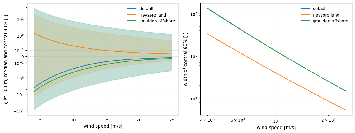
Stability climates for R.KellyGryning, with \(\sigma_\pm\) in \(\mathrm{m}^{-1}\), \(\langle u_*\rangle\) in m/s and \(z_0\) in m.

Climate	\(n_-\)	\(\sigma_+\)	\(\sigma_-\)	\(\langle u_*\rangle\)	\(z_0\)	Source
default	0.60	0.015	0.030	0.30	0.0002	round offshore values
Høvsøre land	0.34	0.0068	0.0116	0.38	0.017	fit with \(p_\pm\) of 2 and 3, three years
IJmuiden offshore	0.69	0.018	0.027	0.30	0.0002	conditional \(z/L\)

examples = (
    ("default", R.KellyGryning(), 0.0002),
    (
        "Høvsøre land",
        R.KellyGryning(
            unstable_fraction=0.34,
            stable_scale=0.0068,
            unstable_scale=0.0116,
            reference_friction_velocity=0.38,
        ),
        0.017,
    ),
    (
        "IJmuiden offshore",
        R.KellyGryning(
            unstable_fraction=0.69, stable_scale=0.018, unstable_scale=0.027
        ),
        0.0002,
    ),
)
fig, axes = plt.subplots(1, 2, figsize=(11.0, 4.2))
for label, model, roughness in examples:
    surface = {"height": 100.0, "roughness_length": roughness}
    low, high = model.bounds(wind_speed, coverage=0.90, **surface)
    median = model.sample(wind_speed, np.full(wind_speed.shape, 0.5), **surface)
    (line,) = axes[0].plot(wind_speed, 100.0 * median, label=label)
    axes[0].fill_between(
        wind_speed, 100.0 * low, 100.0 * high, color=line.get_color(), alpha=0.15
    )
    axes[1].plot(wind_speed, 100.0 * (high - low), label=label)
axes[0].set_yscale("asinh", linear_width=0.1)
axes[0].set(ylabel=r"$\zeta$ at 100 m, median and central 90% [-]")
axes[1].set(xscale="log", yscale="log", ylabel=r"width of central 90% [-]")
for ax in axes:
    ax.set_xlabel("wind speed [m/s]")
    ax.legend(frameon=False)
fig.tight_layout()

Profile and shear

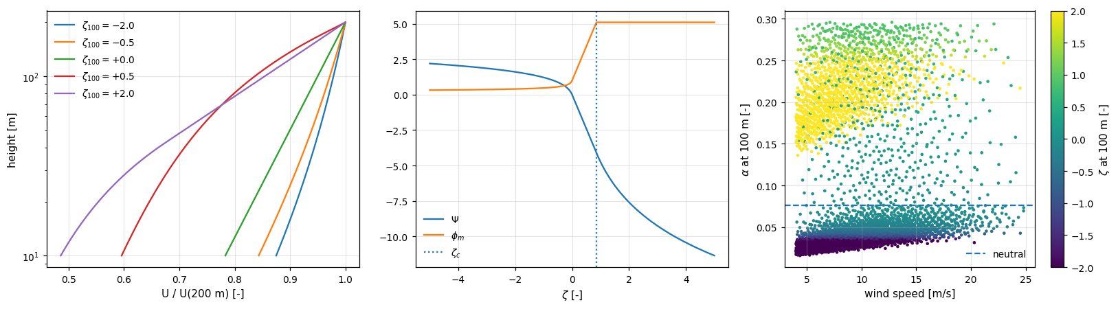
The profile integrates the gradients of Högström (1988),

\[\begin{split}\phi_m = \begin{cases} (1 - 19.3\,\zeta)^{-1/4} & \zeta < 0 \\ 1 + 4.8\,\min(\zeta, \zeta_c) & \zeta \ge 0 \end{cases}, \qquad \Psi(\zeta) = \int_0^{\zeta} \frac{1 - \phi_m(x)}{x}\,\mathrm{d}x,\end{split}\]

held beyond \(\zeta_c = 0.85\) (R.profile.STABLE_LIMIT), where \(\mathrm{Ri} = \zeta\,\phi_h/\phi_m^2\) with \(\phi_h = 0.95 + 7.8\,\zeta\) reaches the critical 0.25. SiteConditions.wind_speed_at(height) evaluates it and the shear exponent at the reference height is

\[\alpha = \frac{\phi_m(z/L)}{\ln(z/z_0) - \Psi(z/L) + \Psi(z_0/L)}.\]

\(z/L\) at 100 m, Høvsøre	0.85 to 2	2 to 5	5 to 20
TI measured	0.063	0.048	0.036
TI, held gradient	0.062	0.050	0.040
TI, no limit	0.061	0.039	0.018
\(\alpha\) measured, 80 to 116.5 m	0.33	0.33	0.29
\(\alpha\), held gradient	0.35	0.28	0.23
\(\alpha\), no limit	0.48	0.67	0.85

height = np.geomspace(10.0, 200.0, 60)
fig, axes = plt.subplots(1, 3, figsize=(15.0, 4.2))
for value in (-2.0, -0.5, 0.0, 0.5, 2.0):
    ratio = np.log(height / 0.0002) - R.profile.stability_correction(
        value * height / 100.0
    )
    axes[0].plot(ratio / ratio[-1], height, label=rf"$\zeta_{{100}}={value:+.1f}$")
axes[0].set(xlabel="U / U(200 m) [-]", ylabel="height [m]", yscale="log")
axes[0].legend(frameon=False)

span = np.linspace(-5.0, 5.0, 400)
axes[1].plot(span, R.profile.stability_correction(span), label=r"$\Psi$")
axes[1].plot(span, R.profile.stability_gradient(span), label=r"$\phi_m$")
axes[1].axvline(R.profile.STABLE_LIMIT, ls=":", label=r"$\zeta_c$")
axes[1].set(xlabel=r"$\zeta$ [-]")
axes[1].legend(frameon=False)

scatter = axes[2].scatter(
    conditions.wind_speed,
    conditions.shear_exponent,
    c=zeta,
    s=4,
    vmin=-2.0,
    vmax=2.0,
)
fig.colorbar(scatter, ax=axes[2], label=r"$\zeta$ at 100 m [-]")
axes[2].axhline(1.0 / np.log(100.0 / 0.0002), ls="--", label="neutral")
axes[2].set(xlabel="wind speed [m/s]", ylabel=r"$\alpha$ at 100 m [-]")
axes[2].legend(frameon=False)
fig.tight_layout()

Charnock roughness

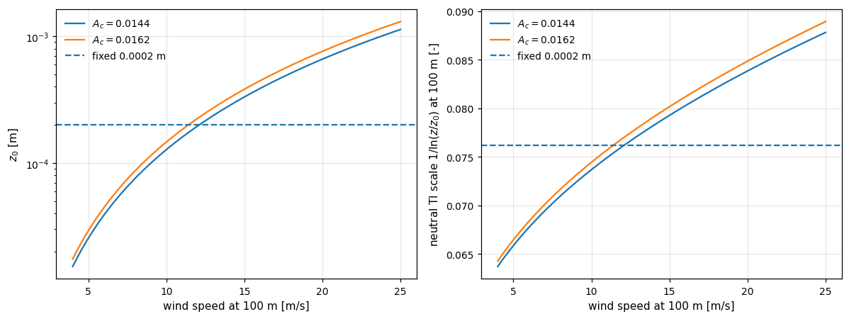
Charnock (1955) set \(z_0 = A_c u_*^2/g\), which with the neutral log law is solved exactly by the lower branch of the Lambert W function (Kelly, 2021),

\[z_0 = \frac{\kappa^2 A_c}{4}\, \frac{U^2/g}{\left[W_{-1}\!\left(-\frac{\kappa U}{2} \sqrt{\frac{A_c}{g z}}\right)\right]^2}.\]

R.Charnock() uses \(A_c = 0.0144\) (Garratt, 1977), and ESDU (1982) recommends 0.0162. In a resource recipe (R.Charnock, {"constant": (0.0144, 0.0162)}) draws a new constant per site.

fig, axes = plt.subplots(1, 2, figsize=(11.0, 4.2))
for constant in (0.0144, 0.0162):
    z0 = R.Charnock(constant).roughness_length(wind_speed, 100.0)
    axes[0].plot(wind_speed, z0, label=rf"$A_c={constant}$")
    axes[1].plot(wind_speed, 1.0 / np.log(100.0 / z0), label=rf"$A_c={constant}$")
axes[0].axhline(2e-4, ls="--", label="fixed 0.0002 m")
axes[1].axhline(1.0 / np.log(100.0 / 2e-4), ls="--", label="fixed 0.0002 m")
axes[0].set(yscale="log", ylabel=r"$z_0$ [m]")
axes[1].set(ylabel=r"neutral TI scale $1/\ln(z/z_0)$ at 100 m [-]")
for ax in axes:
    ax.set_xlabel("wind speed at 100 m [m/s]")
    ax.legend(frameon=False)
fig.tight_layout()

A roughness per sector

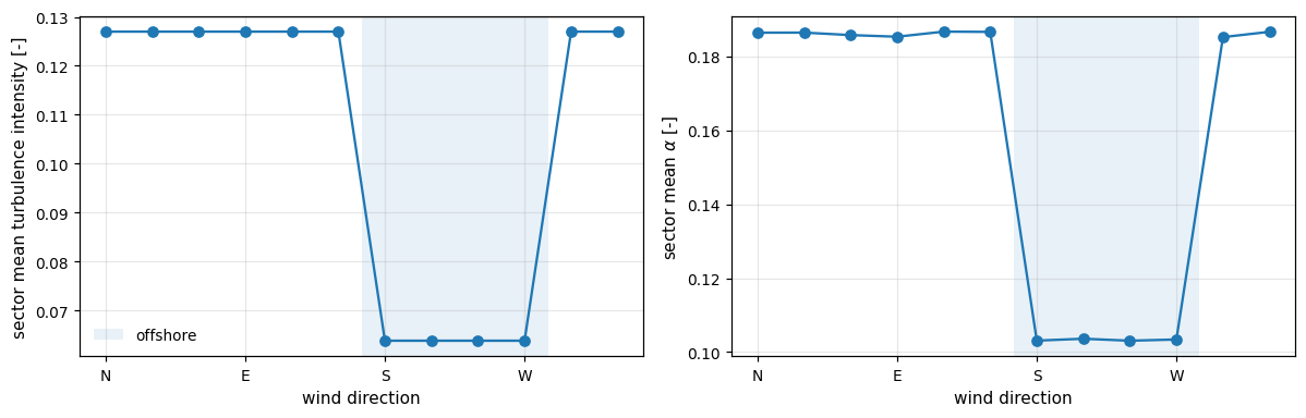
A sequence of one surface per sector, lengths or R.Charnock(), gives each direction its own upwind surface, and every case uses the surface of its sector. Here the four sectors centered from 180 to 270 degrees are offshore. A function that draws a new coastline for every farm is in Describing a population of farms.

coast = tuple(R.Charnock() if 180 <= 30 * i < 300 else 0.1 for i in range(12))
coastal = R.WindResource(roughness_length=coast)
cases = coastal.sample(8192, seed=1)
sector = np.round(cases.wind_direction / 30.0).astype(int) % 12

fig, axes = plt.subplots(1, 2, figsize=(11.0, 3.6))
axes[0].plot(coastal.theta, coastal.sector_turbulence_intensity, marker="o")
axes[0].set(ylabel="sector mean turbulence intensity [-]")
axes[1].plot(
    coastal.theta,
    [cases.shear_exponent[sector == i].mean() for i in range(12)],
    marker="o",
)
axes[1].set(ylabel=r"sector mean $\alpha$ [-]")
for ax in axes:
    ax.axvspan(165.0, 285.0, alpha=0.1, label="offshore")
    ax.set_xticks([0.0, 90.0, 180.0, 270.0], ["N", "E", "S", "W"])
    ax.set_xlabel("wind direction")
axes[0].legend(frameon=False)
fig.tight_layout()

Surface-layer turbulence

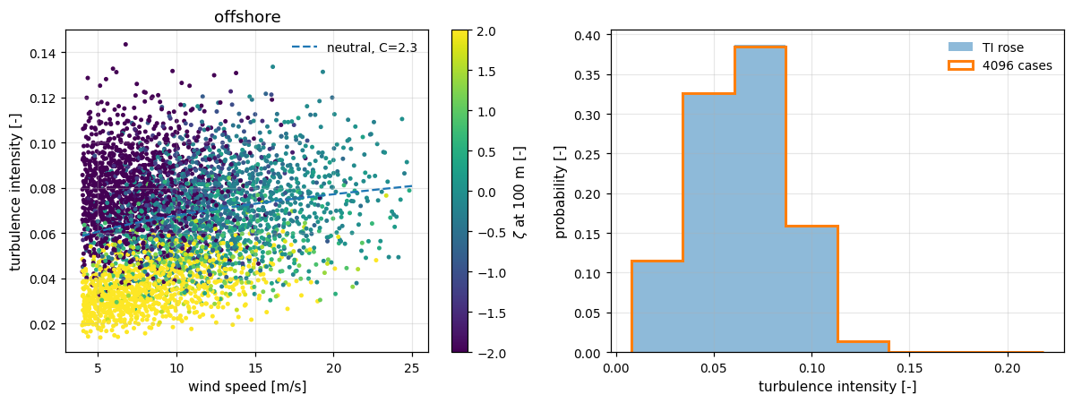
Every case carries \(\sigma_u\) and \(\mathrm{TI} = \sigma_u/U\) from the resource’s turbulence, R.SurfaceLayer. mann=R.Mann() adds the Mann parameters.

\[\sigma_u = C\,u_*, \qquad u_* = \frac{\kappa U}{\ln(z/z_0) - \Psi(z/L) + \Psi(z_0/L)},\]

with \(\Psi\) from the profile above. Kelly (2018) found \(C \approx 2.3\) on average over flat land at Høvsøre from 4 to 25 m/s, the default. coefficient is a number or a bounded scipy.stats distribution drawn per case. At Høvsøre the truncated normal below matches the 99th percentile of \(\sigma_u\) to 7 percent from 4 to 20 m/s, where a fixed \(C\) falls a fifth short.

hovsore_coefficient = stats.truncnorm(-2.36, 3.34, loc=2.3, scale=0.53)
offshore = R.WindResource(
    turbulence=R.SurfaceLayer(hovsore_coefficient),
    roughness_length=R.Charnock(),
    mann=R.Mann(),
)
conditions = offshore.sample(4096, seed=2)
zeta = conditions.stability_parameter(offshore.reference_height)
u = np.linspace(4.0, 25.0, 200)

fig, axes = plt.subplots(1, 2, figsize=(11.0, 4.2))
scatter = axes[0].scatter(
    conditions.wind_speed,
    conditions.turbulence_intensity,
    c=zeta,
    s=5,
    vmin=-2.0,
    vmax=2.0,
)
fig.colorbar(scatter, ax=axes[0], label=r"$\zeta$ at 100 m [-]")
axes[0].plot(
    u,
    2.3 * 0.4 / np.log(100.0 / R.Charnock().roughness_length(u, 100.0)),
    "--",
    label="neutral, C=2.3",
)
axes[0].set(
    xlabel="wind speed [m/s]", ylabel="turbulence intensity [-]", title="offshore"
)
axes[0].legend(frameon=False)

bins = offshore.ti_bins
# The rose is the share of all time, and the cases are given 4 to 25 m/s.
rose = offshore.ti_rose(bins).sum(axis=0)
axes[1].stairs(rose / rose.sum(), bins, fill=True, alpha=0.5, label="TI rose")
axes[1].hist(
    conditions.turbulence_intensity,
    bins=bins,
    weights=conditions.weight,
    histtype="step",
    lw=2,
    label="4096 cases",
)
axes[1].set(xlabel="turbulence intensity [-]", ylabel="probability [-]")
axes[1].legend(frameon=False)
fig.tight_layout()

R.profile.friction_velocity gives the neutral \(u_*\) of a case from its speed, height and roughness. Near neutral stability the cases’ \(\sigma_u / u_*\) is the coefficient they drew, on average its mean.

height = offshore.reference_height
u_star = R.profile.friction_velocity(
    conditions.wind_speed, height, conditions.roughness_length
)
near_neutral = np.abs(conditions.stability_parameter(height)) < 0.02
ratio = conditions.sigma_u[near_neutral] / u_star[near_neutral]
print(f"{near_neutral.sum()} near-neutral cases")
print(
    f"mean sigma_u / u*: {ratio.mean():.2f}, mean C drawn from: "
    f"{hovsore_coefficient.mean():.2f}"
)

80 near-neutral cases
mean sigma_u / u*: 2.33, mean C drawn from: 2.31

Turbulence level

R.SurfaceLayer(intensity=...), one value or one per sector, scales \(\sigma_u\) in sector \(i\) by

\[s_i = \frac{\mathrm{TI}_i}{\left\langle \sigma_u / U \right\rangle_i},\]

the model’s mean over the sector’s Weibull from 4 to 25 m/s, so the spread over speed and stability stays. windIO files keep the mean TI per direction and speed and load back to the same targets. They also keep z0 and the median LMO per speed but not the stability climate, so set stability= again after oowl.load.

target = np.linspace(0.06, 0.12, 12)
resource = R.WindResource(turbulence=R.SurfaceLayer(intensity=target))
cases = resource.sample(8192, seed=1)
sector = np.round(cases.wind_direction / 30.0).astype(int) % 12
print("target ", target.round(3))
print(
    "sampled",
    np.round([cases.turbulence_intensity[sector == i].mean() for i in range(12)], 3),
)

target  [0.06  0.065 0.071 0.076 0.082 0.087 0.093 0.098 0.104 0.109 0.115 0.12 ]
sampled [0.06  0.065 0.071 0.076 0.082 0.087 0.093 0.098 0.104 0.109 0.115 0.12 ]

Mann parameters

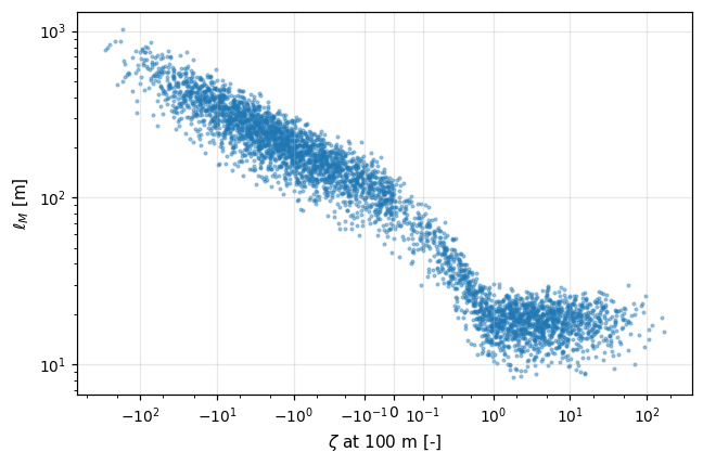
R.Mann gives the length scale of Kelly (2018) from each case’s own profile and a constant anisotropy, 3 as measured by de Maré and Mann (2016) against 3.9 in IEC 61400-1,

\[\ell_M = \frac{\sigma_u}{\mathrm{d}U/\mathrm{d}z} = \frac{C \kappa z}{\phi_m(z/L)}, \qquad \Gamma_M = 3.\]

\(\ell_M\) at 100 m, Høvsøre	neutral	\(z/L\) 0.3 to 0.85	\(z/L\) 0.85 to 5
measured \(\sigma_u\) and shear	55 m	27 m	17 m
profile	89 m	26 m	18 m
spectral fit, Sathe et al. (2013)	40 to 60 m

fig, ax = plt.subplots(figsize=(6.0, 4.0))
ax.scatter(zeta, conditions.mann_length_scale, s=3, alpha=0.4)
ax.set_xscale("asinh", linear_width=0.1)
ax.set_yscale("log")
ax.set(xlabel=r"$\zeta$ at 100 m [-]", ylabel=r"$\ell_M$ [m]")
fig.tight_layout()

TI rose

The TI rose integrates the Weibull density of each sector against the model’s TI distribution, averaged over the stability climate.

von_mises = R.WindResource(direction=R.VonMises(seed=2), n_sectors=24)

fig, axes = plt.subplots(1, 2, figsize=(11, 5), subplot_kw={"projection": "polar"})
von_mises.plot(ax=axes[0], title="wind speed")
von_mises.plot(
    ax=axes[1], variable="turbulence_intensity", title="turbulence intensity"
)
fig.tight_layout()