Sampling with a density

A farm’s count, area and density constrain one geometry, so a sampler takes at most two of them, and Sampling states the rule. The density is one mapping naming area_per_turbine, power_density, minimum_spacing, no pair closer than it, mean_spacing, the mean nearest-neighbor distance, or maximum_spacing, no turbine farther than it from its nearest neighbor, as in density={"minimum_spacing": 800.0}. Uniform and Sobol place turbines at random, so a minimum spacing sizes them by their single closest pair and a mean spacing gives steadier farms. Every density accepts any specification.

given	derived	behavior
n_turbines + area	density	whatever the geometry happens to give
n_turbines + a spacing	area	the boundary is sized so the spacing is met
area + a spacing	n_turbines	the most turbines that hold a minimum or mean, the fewest that hold a maximum

import matplotlib.pyplot as plt
import numpy as np

import oowl
from oowl import boundaries as B
from oowl import layouts as L
from oowl import sampling as SP
from oowl import turbines as T

Ranging the area or holding the spacing

The same count range is drawn twice, once with a ranged area and once with an 800 m spacing. With the area ranged the closest pair wanders, while a held spacing resizes each boundary to fit, so the area becomes a function of the count.

drawn = {
    label: oowl.Sampler(
        B.OffshorePolygon, L.Grid(), n_turbines=(20, 200), seed=3, **sizing
    ).sample(8)
    for label, sizing in (
        ("area=(5, 40) km$^2$", {"area": (5e6, 40e6)}),
        ("minimum spacing 800 m", {"density": {"minimum_spacing": 800.0}}),
    )
}
fig, (left, right) = plt.subplots(1, 2, figsize=(12, 4.5))
for label, farms in drawn.items():
    closest = [farm.metadata["sample"]["closest_pair"] for farm in farms]
    left.plot(closest, "o-", label=label)
    right.plot(
        [farm.n_turbines for farm in farms],
        [farm.boundary.area / 1e6 for farm in farms],
        "o",
        label=label,
    )
left.set(xlabel="scenario", ylabel="closest pair [m]", ylim=(0, None))
right.set(xlabel="turbines", ylabel="area [km$^2$]", ylim=(0, None))
left.legend()
fig.tight_layout()

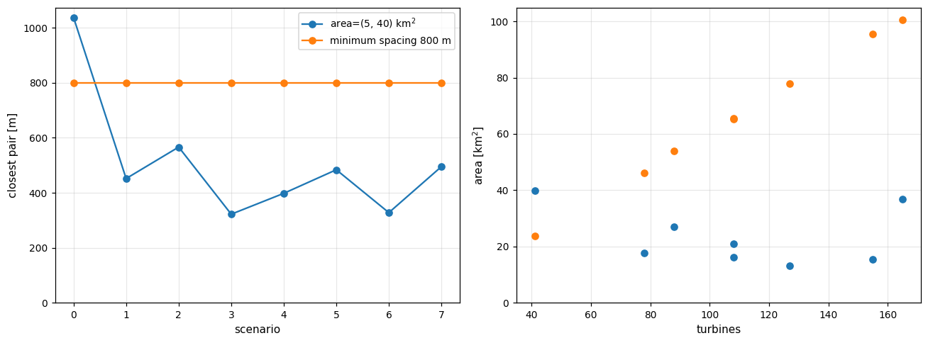
Every layout family is scale-equivariant. For a fixed seed and boundary shape, scaling the area by \(k^2\) scales every distance by \(k\), so one trial draw gives the area a spacing requires. Each farm records minimum_spacing as requested, closest_pair as achieved and area as realized.

A boundary modifier given in meters, such as a Setback or a partition gap, must not scale, so such a boundary is redrawn at the extent that lands on the spacing rather than scaled, as Boundary modifiers describes. A layout can rearrange as its boundary changes and jump over the spacing. The farm just above the spacing is then kept, so no pair is closer than requested, and closest_pair records what was achieved.

record = drawn["minimum spacing 800 m"][0].metadata["sample"]
print(
    {key: round(record[key], 1) for key in ("minimum_spacing", "closest_pair", "area")}
)

{'minimum_spacing': 800.0, 'closest_pair': 800.0, 'area': 23709029.5}

A choice of spacings

A balanced Choice of two spacings splits a population evenly between two size classes.

mixed = oowl.Sampler(
    B.OffshorePolygon,
    L.Grid(60),
    density={"minimum_spacing": SP.Choice([600.0, 1200.0], selection="balanced")},
    seed=4,
)
for farm in mixed.sample(4):
    record = farm.metadata["sample"]
    print(
        f"{record['minimum_spacing']:.0f} m spacing -> {record['area'] / 1e6:.1f} km2"
    )

600 m spacing -> 19.4 km2
1200 m spacing -> 76.0 km2
600 m spacing -> 20.3 km2
1200 m spacing -> 78.6 km2

What a spacing costs, per family

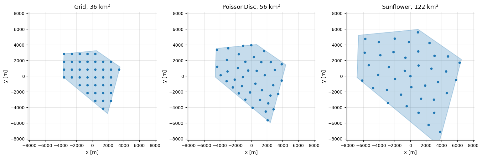
Three families carry 40 turbines at 1000 m on one boundary shape, drawn on shared axes. A lattice packs tightest, and a sunflower, whose arms crowd near the center, needs the largest boundary.

site_shape = B.OffshorePolygon(seed=11)
families = {"Grid": L.Grid, "PoissonDisc": L.PoissonDisc, "Sunflower": L.Sunflower}
spaced = {
    name: oowl.Sampler(
        site_shape, family, n_turbines=40, density={"minimum_spacing": 1000.0}, seed=11
    ).sample()[0]
    for name, family in families.items()
}
reach = 1.15 * max(np.abs(farm.positions).max() for farm in spaced.values())

fig, axes = plt.subplots(1, 3, figsize=(14, 5))
for ax, (name, farm) in zip(axes, spaced.items()):
    farm.plot(ax=ax, s=16, title=f"{name}, {farm.boundary.area / 1e6:.0f} km$^2$")
    ax.set_aspect("equal", adjustable="box")
    ax.set(xlim=(-reach, reach), ylim=(-reach, reach))
fig.tight_layout()

The most turbines a boundary will hold

Given area and minimum_spacing, the layout fills the boundary with the most turbines that fit with no pair closer than it. A layout can carry the spacing itself, as in L.PoissonDisc(density={"minimum_spacing": 1000.0}), and then fills a boundary the same way with or without a sampler. A spacing that fits fewer than two turbines gives a farm of the one that fits.

for name, family in families.items():
    farm = oowl.Sampler(
        site_shape, family, area=40e6, density={"minimum_spacing": 1000.0}, seed=11
    ).sample()[0]
    closest = farm.metadata["sample"]["closest_pair"]
    print(f"{name:<12} {farm.n_turbines:>3} turbines, closest pair {closest:.0f} m")

Grid          43 turbines, closest pair 1010 m
PoissonDisc   27 turbines, closest pair 1018 m
Sunflower     33 turbines, closest pair 1006 m

Asking for all three at once

Count, area and density together over-constrain a farm and are refused when the sampler is built, and so are two densities. A sampler’s density sizes one farm, so for a cluster give it to the layout, as in L.Grid(density={"minimum_spacing": 800.0}), which fills every member to it, or put per-member sizing in a farm configuration, as Drawing, streaming and replaying a population does. A count and a spacing with fewer than two turbines have nothing to scale and are reported when drawn.

To keep a farm of fixed count and area at least 800 m apart, check it with requirements={"spacing": (800.0, None)} instead, which sizes nothing.

for kwargs in (
    {"n_turbines": 60, "area": 40e6, "density": {"minimum_spacing": 800.0}},
    {"density": {"area_per_turbine": 6e5, "minimum_spacing": 800.0}},
    {"n_farms": 3, "density": {"minimum_spacing": 800.0}},
):
    try:
        oowl.Sampler(B.OffshorePolygon, L.Grid, **kwargs)
    except ValueError as exc:
        print(exc)

n_turbines, area and minimum_spacing over-constrain the same geometry. Give any two and the third follows, or keep the spacing as a floor the farm is checked against with Sampler(requirements={'spacing': (minimum, None)})
density takes one of area_per_turbine, power_density, minimum_spacing, mean_spacing, maximum_spacing, got 2
minimum_spacing sizes a single farm and cannot size a cluster. Put the specification in a farm configuration instead, as in configuration={'boundary': OffshorePolygon, 'layout': PoissonDisc, 'n_turbines': 40, 'density': {'minimum_spacing': 600.0}}, which is drawn once per member

Densities from the turbine

A power_density in watts per square meter of installed capacity turns into a count through the turbine’s rated power, and a spacing given as SP.RotorDiameters(7) turns into meters through its rotor diameter, the largest when a farm mixes turbines. A drawn turbine then carries its density with it. A mean spacing works for every layout too.

turbine = T.Idealized(15e6, 240.0, 150.0, 0.45)
for density in (
    {"power_density": 6.0},
    {"minimum_spacing": SP.RotorDiameters(7)},
    {"mean_spacing": 1000.0},
):
    farm = oowl.Sampler(
        site_shape, L.Grid, area=60e6, turbines=turbine, seed=11, density=density
    ).sample()[0]
    print(
        f"{density}: {farm.n_turbines} turbines, closest {farm.minimum_spacing():.0f} m"
    )

{'power_density': 6.0}: 24 turbines, closest 1698 m
{'minimum_spacing': RotorDiameters(7)}: 24 turbines, closest 1688 m
{'mean_spacing': 1000.0}: 63 turbines, closest 1005 m