Wind resources

A resource gives each direction sector a probability and a Weibull speed distribution. Stability and turbulence adds the surface, stability and turbulence of each case, and sample draws the cases. Three uses cover most studies. One site sampled many times describes that site.

import matplotlib.pyplot as plt
import numpy as np
from scipy import stats
from scipy.special import i0

import oowl
from oowl import resources as R

site = R.WindResource(mean_wind_speed=9.0, roughness_length=R.Charnock())
cases = site.sample(1000, seed=1)

One case from each of many drawn sites describes the range of real sites.

recipe = (
    R.WindResource,
    {
        "direction": R.VonMises,
        "mean_wind_speed": (5.0, 11.0),
        "roughness_length": stats.loguniform(2e-4, 1.0),
    },
)
sites = oowl.Sampler(resource=recipe, seed=1).sample(1000)
cases = [site.sample(1, seed=index) for index, site in enumerate(sites)]

A coverage design spans the conditions any site may produce, see Coverage design.

design = R.Dimitrov()
cases = design.sample(1000, seed=1)

Direction

Every resource divides the compass into \(n\) equal sectors centered at

\[\theta_i = \frac{2\pi i}{n}, \qquad i = 0, \ldots, n - 1,\]

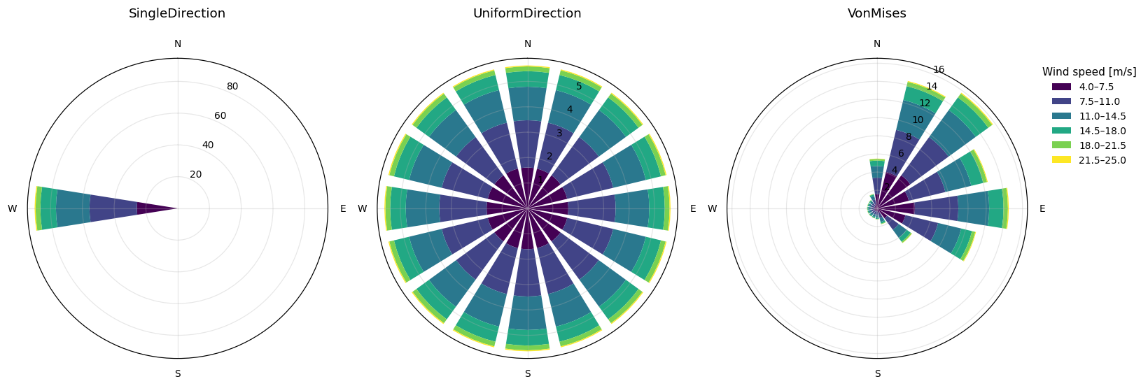
with probabilities \(p_i \ge 0\) and \(\sum_i p_i = 1\), 0° north and 90° east. Each \(p_i\) is the mass of its sector, not a density at its center. R.SingleDirection turns the sectors so one is centered on its direction.

A resource’s direction sets the \(p_i\), R.UniformDirection() by default.

climate = {"n_sectors": 16, "mean_wind_speed": 9.5, "weibull_k": 2.3}
models = {
    "SingleDirection": R.WindResource(direction=R.SingleDirection(270.0), **climate),
    "UniformDirection": R.WindResource(**climate),
    "VonMises": R.WindResource(direction=R.VonMises(n_modes=2, seed=2), **climate),
}

fig, axes = plt.subplots(1, 3, figsize=(15, 5), subplot_kw={"projection": "polar"})
for index, (ax, (name, resource)) in enumerate(zip(axes, models.items())):
    resource.plot(ax=ax, legend=index == 2, title=name)
fig.tight_layout()

Von Mises directions

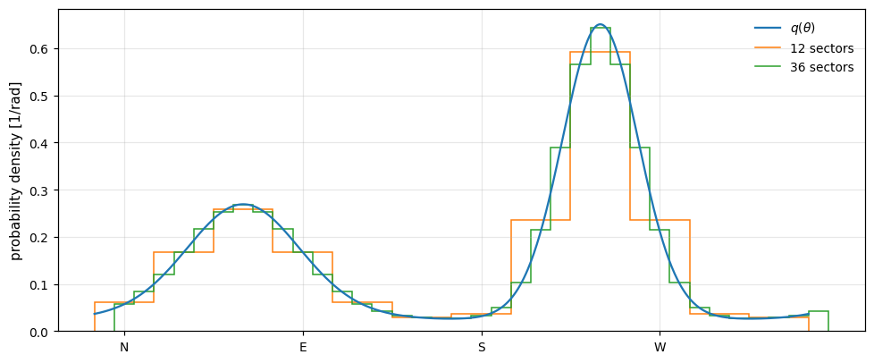
VonMises is the mixture of von Mises distributions (Mardia and Jupp, 2000) that Carta et al. (2008) fit to wind directions, on a uniform background \(b\), the mode of zero concentration. Mode \(j\) has mean direction \(\mu_j\), concentration \(\kappa_j\), larger for a narrower mode, and weight \(w_j\), the weights summing to \(1 - b\),

\[q(\theta) = \frac{b}{2\pi} + \sum_j w_j\, \frac{\exp\left[\kappa_j\cos(\theta - \mu_j)\right]}{2\pi I_0(\kappa_j)}, \qquad p_i = \int_{\theta_i - \Delta/2}^{\theta_i + \Delta/2} q(\theta)\,d\theta.\]

Modes are (direction, concentration, weight) tuples, or drawn by seed. The sector count sets the resolution, not the model. The sectors here also differ in speed, since weibull_a gives each its own Weibull scale.

theta = np.arange(24) * 15.0
von_mises = R.WindResource(
    direction=R.VonMises(
        modes=[(240.0, 9.0, 1.0), (60.0, 4.0, 0.6)], background_fraction=0.15
    ),
    n_sectors=24,
    weibull_a=9.5 + 1.5 * np.cos(np.deg2rad(theta - 240.0)),
    weibull_k=2.4,
)


def density(angle):
    weights = np.array([1.0, 0.6])
    weights = 0.85 * weights / weights.sum()
    q = np.full_like(angle, 0.15 / (2.0 * np.pi))
    for (mu, kappa), weight in zip([(240.0, 9.0), (60.0, 4.0)], weights):
        q += (
            weight
            * np.exp(kappa * np.cos(angle - np.deg2rad(mu)))
            / (2 * np.pi * i0(kappa))
        )
    return q


direction = np.linspace(-15.0, 345.0, 721)
fig, ax = plt.subplots(figsize=(9.0, 3.8))
ax.plot(direction, density(np.deg2rad(direction)), label=r"$q(\theta)$")
for n in (12, 36):
    width = 360.0 / n
    edges = np.arange(n + 1) * width - 0.5 * width
    density_n = von_mises.direction.probabilities(n) / np.deg2rad(width)
    ax.stairs(density_n, edges, label=f"{n} sectors")
ax.set_xticks([0.0, 90.0, 180.0, 270.0], ["N", "E", "S", "W"])
ax.set_ylabel("probability density [1/rad]")
ax.legend(frameon=False)
fig.tight_layout()

Elliptical roses

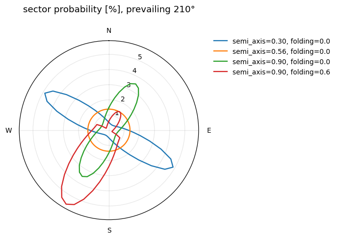
Elliptical is the ellipse rose of Hart (2025). Directions follow an ellipse of unit area whose semi_axis lies along the prevailing axis. semi_axis \(= 1/\sqrt{\pi}\) is a circle and uniform, a longer one concentrates probability along the prevailing axis, a shorter one across it, and folding moves the opposite half toward it.

fig = plt.figure(figsize=(6.0, 5.5))
ax = fig.add_subplot(projection="polar")
ax.set_theta_zero_location("N")
ax.set_theta_direction(-1)
for semi_axis, folding in [
    (0.30, 0.0),
    (1.0 / np.sqrt(np.pi), 0.0),
    (0.90, 0.0),
    (0.90, 0.6),
]:
    resource = R.WindResource(
        direction=R.Elliptical(semi_axis=semi_axis, folding=folding, direction=210.0),
        n_sectors=72,
    )
    p = resource.probability
    ax.plot(
        np.deg2rad(np.append(resource.theta, 360.0)),
        100.0 * np.append(p, p[0]),
        label=f"semi_axis={semi_axis:.2f}, folding={folding}",
    )
ax.set_thetagrids([0, 90, 180, 270], labels=["N", "E", "S", "W"])
ax.set_title("sector probability [%], prevailing 210°", pad=20)
ax.legend(loc="upper left", bbox_to_anchor=(1.05, 1.05), frameon=False)
fig.tight_layout()

Speed

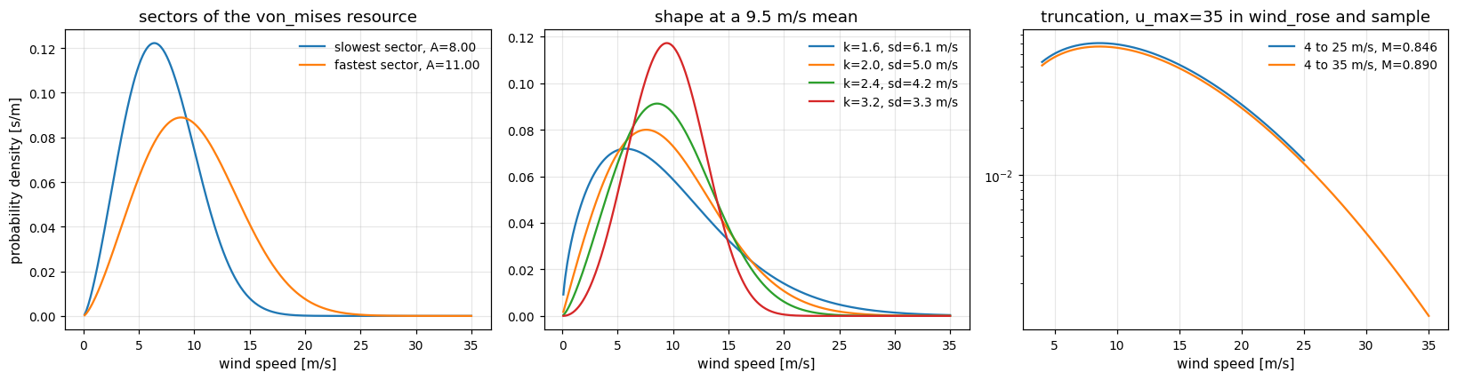
Given sector \(i\) the speed is Weibull (Weibull, 1951),

\[F_i(u) = 1 - \exp\left[-\left(\frac{u}{A_i}\right)^{k_i}\right], \qquad A_i = \frac{\bar U_i}{\Gamma(1 + 1/k_i)}.\]

The mean, the spread and the rose of sector \(i\) and speed bin \([l_j, h_j]\) are exact,

\[\bar U = \sum_i p_i \bar U_i, \qquad \sigma_U^2 = \sum_i p_i A_i^2\,\Gamma(1 + 2/k_i) - \bar U^2, \qquad P(i, j) = p_i\left[F_i(h_j) - F_i(l_j)\right].\]

mean_wind_speed sets \(\bar U\), or weibull_a sets \(A_i\) and \(\bar U\) follows. \(P(i, j)\) is the share of all time, calm included, so wind_rose sums to \(M = \sum_i p_i\left[F_i(u_{\max}) - F_i(u_{\min})\right]\), the share of time in \([u_{\min}, u_{\max}]\), 4 to 25 m/s by default. Annual energy is 8760 h times the sum of the rose times the power in each bin. u_min=0 covers calm air, and dividing by \(M\) gives the rose given a speed in the range, which the sampled cases follow. Each case records \(M\) as metadata["in_range_fraction"].

means = von_mises.sector_mean_wind_speed
rose = von_mises.wind_rose()
print(f"rose sums to {rose.sum():.4f}, the share of time in 4 to 25 m/s")
print(f"from calm to 25 m/s {von_mises.wind_rose(u_min=0.0).sum():.4f}")
print(
    f"mean {von_mises.mean_wind_speed:.2f} m/s, "
    f"sd {von_mises.wind_speed_standard_deviation:.2f} m/s"
)

rose sums to 0.8832, the share of time in 4 to 25 m/s
from calm to 25 m/s 0.9996
mean 8.72 m/s, sd 4.07 m/s

Sector densities, the shape at a fixed mean, and the truncation interval.

def weibull_pdf(u, a, k):
    return (k / a) * (u / a) ** (k - 1.0) * np.exp(-((u / a) ** k))


u = np.linspace(0.1, 35.0, 400)
fig, axes = plt.subplots(1, 3, figsize=(15.0, 4.0))
for label, index in (("slowest", np.argmin(means)), ("fastest", np.argmax(means))):
    a, k = von_mises.weibull_a[index], von_mises.weibull_k[index]
    axes[0].plot(u, weibull_pdf(u, a, k), label=f"{label} sector, A={a:.2f}")
axes[0].set_title("sectors of the von_mises resource")

for k in (1.6, 2.0, 2.4, 3.2):
    resource = R.WindResource(mean_wind_speed=9.5, weibull_k=k)
    sd = resource.wind_speed_standard_deviation
    axes[1].plot(
        u, weibull_pdf(u, resource.weibull_a[0], k), label=f"k={k}, sd={sd:.1f} m/s"
    )
axes[1].set_title("shape at a 9.5 m/s mean")

windy = R.WindResource(mean_wind_speed=12.0, weibull_k=1.8)
a, k = windy.weibull_a[0], windy.weibull_k[0]
for u_max in (25.0, 35.0):
    speed = np.linspace(4.0, u_max, 300)
    mass = np.exp(-((4.0 / a) ** k)) - np.exp(-((u_max / a) ** k))
    axes[2].plot(
        speed,
        weibull_pdf(speed, a, k) / mass,
        label=f"4 to {u_max:.0f} m/s, M={mass:.3f}",
    )
axes[2].set_yscale("log")
axes[2].set_title("truncation, u_max=35 in wind_rose and sample")
for ax in axes:
    ax.set_xlabel("wind speed [m/s]")
    ax.legend(frameon=False)
axes[0].set_ylabel("probability density [s/m]")
fig.tight_layout()

Sampling cases

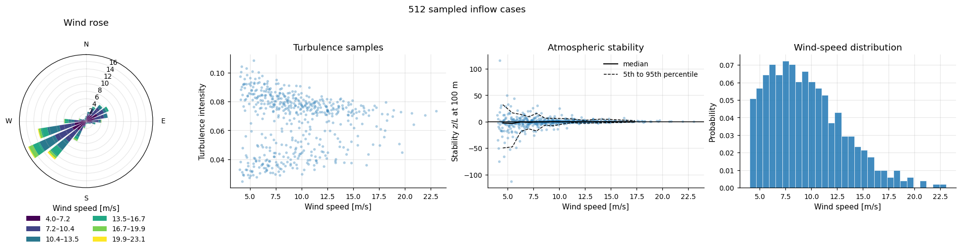
One scrambled Sobol point \(\mathbf q\) (Sobol’, 1967) becomes one case, each link the inverse CDF of one coordinate given the links before it.

1. \(q_0\) picks the sector from the in-range weights \(p_i\left[F_i(u_{\max}) - F_i(u_{\min})\right]/M\).

2. \(q_1\) picks the speed, \(U = A_i\left[-\ln(1 - F)\right]^{1/k_i}\) with \(F = F_i(u_{\min}) + q_1\left[F_i(u_{\max}) - F_i(u_{\min})\right]\).

3. The roughness follows from the speed, see Stability and turbulence.

4. \(q_2\) gives \(1/L\) given speed and roughness, see Stability and turbulence.

5. \(q_3\) gives \(\sigma_u\), see Stability and turbulence.

6. The shear exponent follows from the profile.

Designs of Coverage design add one coordinate per variable they draw. Each case weighs \(1/N\) of the time in range, whose share of all time is metadata["in_range_fraction"].

conditions = von_mises.sample(512, seed=1)
print(
    f"weights sum to {conditions.weight.sum():.3f}, in range {conditions.metadata['in_range_fraction']:.3f}"
)
conditions.plot(title="512 sampled inflow cases");

weights sum to 1.000, in range 0.883

Global Wind Atlas

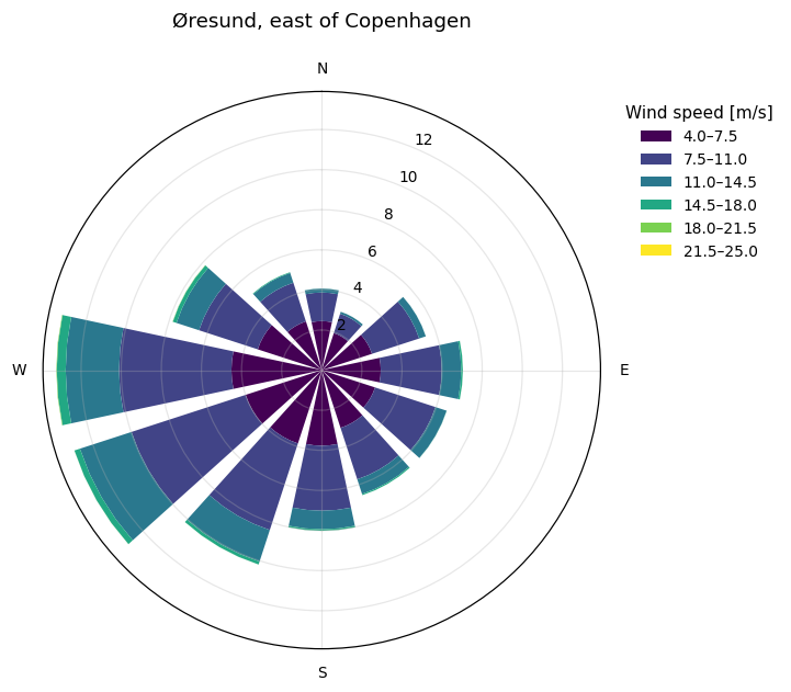
GWA downloads the Global Wind Climate libfile of a point from the Global Wind Atlas and interpolates its Weibull \(A\) and \(k\) linearly in \(\ln z_0\) and in height, and its sector frequencies linearly in \(\ln z_0\) (WAsP methodology). libfile_path= reads a saved libfile instead of the network. This page reads oresund.lib, saved from the atlas for this point, so it builds offline and gives the same climate a download does.

site = R.GWA(
    latitude=55.7,
    longitude=12.7,
    roughness_length=0.05,
    reference_height=100.0,
    libfile_path="oresund.lib",
)
print(site)
site.plot(title="Øresund, east of Copenhagen");

GWA(latitude=55.7, longitude=12.7, roughness_length=0.05, reference_height=100, stability=KellyGryning(unstable_fraction=0.6, stable_scale=0.015, unstable_scale=0.03, reference_friction_velocity=0.3, stable_exponent=2, unstable_exponent=3, fraction_friction_velocity=None), turbulence=SurfaceLayer(coefficient=2.3, intensity=None), mann=None, timeout=30, libfile_path='oresund.lib')

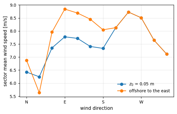
One roughness per atlas sector reads each sector at its own \(z_0\), for a site whose upwind surface changes with direction. Here the sectors from north to south through east are offshore. The frequencies are renormalized.

coast = tuple(0.0002 if 30 * i <= 180 else 0.05 for i in range(12))
coastal = R.GWA(
    latitude=55.7,
    longitude=12.7,
    roughness_length=coast,
    reference_height=100.0,
    libfile_path="oresund.lib",
)
fig, ax = plt.subplots(figsize=(6.0, 3.6))
ax.plot(site.theta, site.sector_mean_wind_speed, marker="o", label="$z_0$ = 0.05 m")
ax.plot(
    coastal.theta,
    coastal.sector_mean_wind_speed,
    marker="o",
    label="offshore to the east",
)
ax.set_xticks([0.0, 90.0, 180.0, 270.0], ["N", "E", "S", "W"])
ax.set(xlabel="wind direction", ylabel="sector mean wind speed [m/s]")
ax.legend(frameon=False);