Turbine models#

A turbine is rotor geometry plus power and thrust-coefficient curves. Idealized and Controlled generate their curves from design parameters and Tabulated interpolates supplied curves. All three are configured below as the same 15 MW machine on a 240 m rotor. Attaching turbines to a farm attaches a model to a farm and windIO interchange saves one.

A turbine definition needs only the turbines module.

from dataclasses import replace

import matplotlib.pyplot as plt
import numpy as np

from oowl import turbines as T

Rotor power and the Betz limit#

The analytical models, Idealized and Controlled, work from rotor area

\[ A_r=\frac{\pi D^2}{4} \]

and electrical power

\[ P(U)=\eta_g\,\frac12\rho A_r C_P(U)\,U^3, \]

where \(\eta_g\) is generator efficiency. OOWL rejects one outside \(0<C_{P,\max}\le16/27\), the ideal actuator-disc Betz limit. A Tabulated turbine takes its power curve as given. The actuator-disc relations behind the analytical models are discussed by Sørensen in “Generalized analytical body force model for actuator disc computations of wind turbines”, Wind Energy Science 8 (2023), 1017-1027.

Idealized#

Rated speed follows from the rating and the rotor.

\[ U_r=\left( \frac{P_r}{\eta_g\,\tfrac12\rho A_r C_{P,\max}} \right)^{1/3}. \]

The power coefficient is constant up to rated and falls as \(U^{-3}\) above it.

\[\begin{split} C_P(U)= \begin{cases} 0, & U<U_{\mathrm{in}}\ \text{or}\ U>U_{\mathrm{out}},\\ C_{P,\max}, & U_{\mathrm{in}}\le U\le U_r,\\ C_{P,\max}(U_r/U)^3, & U_r<U\le U_{\mathrm{out}}. \end{cases} \end{split}\]

Below rated, \(C_T\) is the configured ct_rated. Above rated, OOWL maps \(C_P\) to an axial-induction proxy

\[ a(C_P)=\frac23\left[1- \cos\left(\frac13\arccos\left(1-2\frac{C_P}{16/27}\right)\right) \right] \]

and rescales \(a(1-a)\) so the curve meets the configured rated thrust.

\[ C_T(U)=C_{T,r}\, \frac{a(U)\left[1-a(U)\right]}{a_r\left(1-a_r\right)}. \]

The optional ct_idle and ct_parked set idle and parked thrust. They default to zero and to the terminal operating \(C_T\).

idealized = T.Idealized(
    rated_power=15e6,
    rotor_diameter=240.0,
    hub_height=150.0,
    cp_max=0.46184,
    ct_rated=0.7783,
    generator_efficiency=0.95756,
    cutin_wind_speed=3.0,
    ct_idle=0.06,
    ct_parked=0.18,
    name="15 MW idealized",
)

print(idealized)
print(f"rotor area: {idealized.rotor_area:,.0f} m^2")
print(f"derived rated wind speed: {idealized.rated_wind_speed:.2f} m/s")

Idealized(rated_power=1.5e+07, rotor_diameter=240, hub_height=150, cp_max=0.46184, ct_rated=0.7783, air_density=1.225, generator_efficiency=0.95756, cutin_wind_speed=3, cutout_wind_speed=25, ct_idle=0.06, ct_parked=0.18, name='15 MW idealized')
rotor area: 45,239 m^2
derived rated wind speed: 10.70 m/s

Controlled#

Controlled tracks the optimal tip-speed ratio \(\lambda_*\) with a variable-speed rotor. Rotor speed is held between minimum_rotor_speed and maximum_tip_speed,

\[ \Omega(U)=\operatorname{clip}\left(\frac{\lambda_*U}{R},\ \Omega_{\min},\ \frac{v_{\mathrm{tip}}}{R}\right), \]

which makes the realized ratio \(\lambda=\Omega R/U\). Thrust and power both follow one axial induction factor

\[ a(U)=a_*\left(\frac{\lambda}{\lambda_*}\right)^{\kappa}, \]

where \(a_*\) gives ct_optimal and \(\kappa\) is induction_exponent. Thrust is the momentum value \(C_T=4a(1-a)\), with the empirical correction of Buhl (2005) above \(a=0.4\). The power coefficient is

\[ C_P=\eta_b\,\min\left[4a(1-a)^2,\ 4a_*(1-a_*)^2\right] \exp\left[-0.8\left|\frac{\lambda}{\lambda_*}-1\right|^3\right], \]

with the blade efficiency \(\eta_b\) set so that \(C_P=C_{P,\max}\) at \(\lambda_*\). Extra induction adds thrust but no power. Rated speed is the first speed at which power reaches \(P_r\). Above it the blades pitch to hold rated power and \(a\) falls with \(C_P\).

At the minimum rotor speed, near cut-in, the rotor over-induces and thrust rises. At the tip-speed limit it falls before rated. ct_peak_shaving caps the thrust, thrust_slope tilts the design thrust with wind speed below rated, and turbulence_smoothing rounds the knee at rated as in measured curves. The loss constants are synthetic, not a blade-element model. This turbine keeps the default idle and parked thrust.

controlled = T.Controlled(
    rated_power=15e6,
    rotor_diameter=240.0,
    hub_height=150.0,
    cp_max=0.46184,
    optimal_tip_speed_ratio=9.0,
    minimum_rotor_speed=5.0,
    maximum_tip_speed=95.0,
    ct_optimal=0.7783,
    induction_exponent=0.05,
    generator_efficiency=0.95756,
    cutin_wind_speed=3.0,
    name="15 MW controlled",
)

print(controlled)
print(f"derived rated wind speed: {controlled.rated_wind_speed:.2f} m/s")

Controlled(rated_power=1.5e+07, rotor_diameter=240, hub_height=150, cp_max=0.46184, optimal_tip_speed_ratio=9, minimum_rotor_speed=5, maximum_tip_speed=95, ct_optimal=0.7783, induction_exponent=0.05, ct_peak_shaving=None, thrust_slope=0, turbulence_smoothing=0, air_density=1.225, generator_efficiency=0.95756, cutin_wind_speed=3, cutout_wind_speed=25, ct_idle=None, ct_parked=None, name='15 MW controlled')
derived rated wind speed: 10.70 m/s

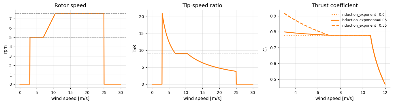
Rotor speed is clipped below 7 m/s and from 10.6 m/s, just before rated. The right panel compares induction exponents. This turbine uses 0.05, which matches the nearly flat thrust of the reference table below. Many published curves rise more steeply toward cut-in, which the default of 0.35 follows.

speeds = np.linspace(0.0, 30.0, 601)

maximum_rpm = controlled.maximum_tip_speed / controlled.rotor_radius * 60 / (2 * np.pi)
low_wind = np.linspace(3.0, 12.0, 181)

fig, axes = plt.subplots(1, 3, figsize=(12.5, 3.4))
axes[0].plot(speeds, controlled.rotor_speed(speeds), color="C1", lw=2)
axes[0].axhline(controlled.minimum_rotor_speed, color="C7", ls="--", lw=1)
axes[0].axhline(maximum_rpm, color="C7", ls="--", lw=1)
axes[1].plot(speeds, controlled.tip_speed_ratio(speeds), color="C1", lw=2)
axes[1].axhline(controlled.optimal_tip_speed_ratio, color="C7", ls="--", lw=1)
for exponent, style in ((0.0, ":"), (0.05, "-"), (0.35, "--")):
    variant = replace(controlled, induction_exponent=exponent)
    axes[2].plot(
        low_wind,
        variant.ct(low_wind),
        color="C1",
        ls=style,
        lw=2,
        label=f"induction_exponent={exponent}",
    )
axes[2].legend(frameon=False, fontsize=8)
panels = zip(
    axes,
    ("Rotor speed", "Tip-speed ratio", "Thrust coefficient"),
    ("rpm", "TSR", "$C_T$"),
)
for ax, title, ylabel in panels:
    ax.set(title=title, xlabel="wind speed [m/s]", ylabel=ylabel)
    ax.grid(True)
    ax.spines[["top", "right"]].set_visible(False)
fig.tight_layout()

../_images/ce6f7474041db8574b98278b07162162633642464ca115a627764e0ed795bcd4.png

Tabulated#

Tabulated interpolates a measured curve linearly and returns zero outside its range, with cut-in, cut-out and rated speed read off the table. It has no cp method. Here it holds published reference rows for the same 15 MW machine.

# The IEA-15-240-RWT rows hold wind speed, power, CP and CT.
reference = np.array(
    [
        [3.0000, 0.0431, 0.0595, 0.8023],
        [4.0679, 0.6072, 0.3364, 0.7779],
        [5.0064, 1.4011, 0.4164, 0.7842],
        [6.1530, 2.8247, 0.4522, 0.7859],
        [6.9655, 4.1802, 0.4613, 0.7818],
        [8.1767, 6.7670, 0.4616, 0.7783],
        [9.3856, 10.2339, 0.4616, 0.7783],
        [10.6594, 15.0000, 0.4618, 0.7718],
        [11.6993, 15.0000, 0.3493, 0.4616],
        [14.7781, 15.0000, 0.1733, 0.2074],
        [20.0299, 15.0000, 0.0696, 0.0827],
        [25.0000, 15.0000, 0.0358, 0.0442],
    ]
)
reference_speed, reference_power, reference_cp, reference_ct = reference.T

measured = T.Tabulated(
    rotor_diameter=240.0,
    hub_height=150.0,
    wind_speeds=reference_speed,
    power_values=reference_power * 1e6,
    ct_values=reference_ct,
    name="15 MW measured",
)
tabulated_band = (speeds >= measured.cutin_wind_speed) & (
    speeds <= measured.cutout_wind_speed
)
measured_cp = np.where(
    tabulated_band, np.interp(speeds, reference_speed, reference_cp), 0.0
)

print(measured)
band = f"{measured.cutin_wind_speed:.1f} to {measured.cutout_wind_speed:.1f} m/s"
print(f"operating range read off the table: {band}")
print(f"rated wind speed read off the table: {measured.rated_wind_speed:.2f} m/s")

Tabulated(rotor_diameter=240, hub_height=150, wind_speeds=[3.0, 4.0679, 5.0064, 6.153, 6.9655, 8.1767, 9.3856, 10.6594, 11.6993, 14.7781, 20.0299, 25.0], power_values=[43100.0, 607200.0, 1401100.0, 2824700.0, 4180200.0, 6767000.0, 10233900.0, 15000000.0, 15000000.0, 15000000.0, 15000000.0, 15000000.0], ct_values=[0.8023, 0.7779, 0.7842, 0.7859, 0.7818, 0.7783, 0.7783, 0.7718, 0.4616, 0.2074, 0.0827, 0.0442], name='15 MW measured', rated_power=1.5e+07)
operating range read off the table: 3.0 to 25.0 m/s
rated wind speed read off the table: 10.66 m/s

Comparing the three models#

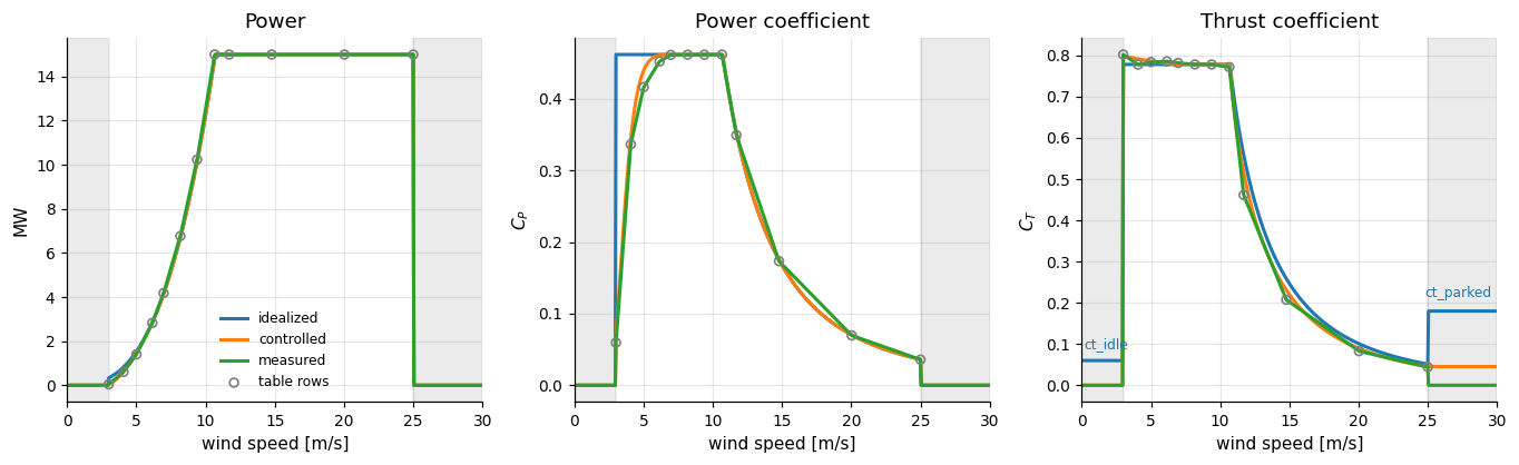
Shaded bands mark the idle and parked states.

The idealized \(C_P\) jumps to its plateau at cut-in, a 0.33 MW power step, and overshoots the table on either side of rated. Tip-speed-ratio losses bring the controlled model back onto the measured curve.
Above the shared rated speed the controlled thrust follows the pitching rotor’s induction and sits closer to the table than the idealized mapping.
Parked, the idealized turbine holds 0.18 and the controlled turbine about 0.05. Idle, they hold 0.06 and zero.
The measured curve is zero in both bands.

models = (
    ("idealized", idealized, "C0"),
    ("controlled", controlled, "C1"),
    ("measured", measured, "C2"),
)
knots = dict(s=26, facecolors="none", edgecolors="C7", lw=1.1, zorder=4)

fig, axes = plt.subplots(1, 3, figsize=(12.5, 3.9), sharex=True)
for label, turbine, color in models:
    power_mw = np.asarray(turbine.power(speeds)) / 1e6
    axes[0].plot(speeds, power_mw, color=color, lw=2, label=label)
    axes[2].plot(speeds, turbine.ct(speeds), color=color, lw=2)
for label, turbine, color in models[:2]:
    axes[1].plot(speeds, turbine.cp(speeds), color=color, lw=2)
axes[1].plot(speeds, measured_cp, color="C2", lw=2)

axes[0].scatter(reference_speed, reference_power, label="table rows", **knots)
axes[1].scatter(reference_speed, reference_cp, **knots)
axes[2].scatter(reference_speed, reference_ct, **knots)
axes[2].annotate("ct_idle", (0.2, 0.09), fontsize=8, color="C0")
axes[2].annotate("ct_parked", (29.6, 0.215), fontsize=8, color="C0", ha="right")

titles = ("Power", "Power coefficient", "Thrust coefficient")
ylabels = ("MW", "$C_P$", "$C_T$")
for ax, title, ylabel in zip(axes, titles, ylabels):
    ax.axvspan(0.0, idealized.cutin_wind_speed, color="C7", alpha=0.15)
    ax.axvspan(idealized.cutout_wind_speed, speeds[-1], color="C7", alpha=0.15)
    ax.set(title=title, xlabel="wind speed [m/s]", ylabel=ylabel)
    ax.grid(True)
    ax.spines[["top", "right"]].set_visible(False)
axes[0].set_xlim(0.0, speeds[-1])
axes[0].legend(frameon=False, fontsize=8)
fig.tight_layout()

../_images/7c8d0158d26b64d885be47cd33b3f0403487e8f05e6074ae1db3d2e9487e5f6e.png

These models omit yaw and tilt losses, air-density variation, aeroelastic loads, dynamic control, availability, degradation, acoustics and certification load cases, which belong to standards such as IEC 61400-1.

Turbine models

Contents