Layout families

A layout family turns a boundary and a turbine count into positions. It evaluates no wakes, cabling or yield, so a layout is a spatial hypothesis, not an optimum.

import matplotlib.pyplot as plt
import numpy as np

import oowl
from oowl import boundaries as B
from oowl import layouts as L
from oowl import modifiers as M
from oowl import strings as S

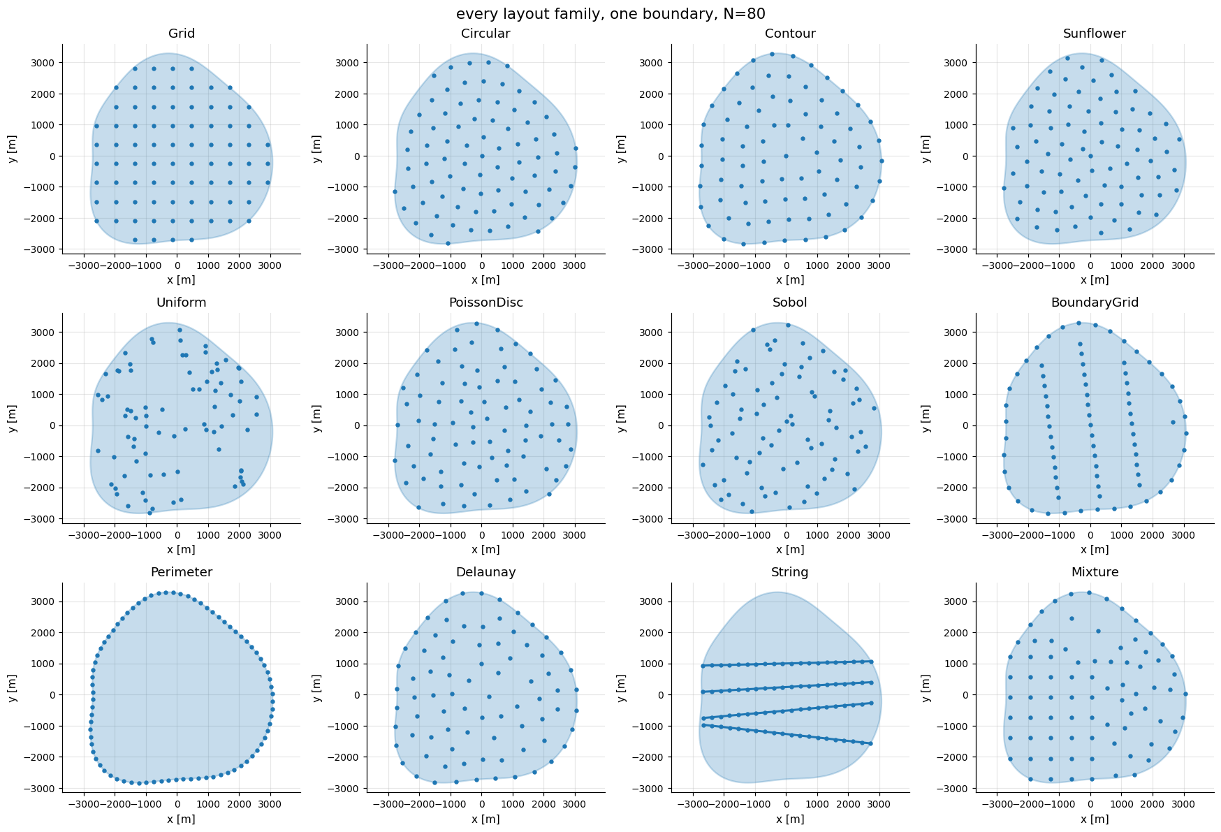
Twelve families share one boundary and n = 80.

1. Candidate fields (Grid, Circular, Contour, Sunflower) scale a field, clip it and select exactly \(N\).

2. Finite patterns (PoissonDisc, String) build \(N\) normalized points and fit the largest rigid scale and translation inside the boundary. String follows a string guide (String layouts).

3. Boundary-conforming families (BoundaryGrid, Perimeter, Delaunay) work in realized coordinates.

Uniform and Sobol draw positions inside the boundary without a fit. Mixture lays families out in weighted cells of one farm (Combining layout families).

n = 80
boundary = B.SmoothBlob(area=np.pi * 3000**2, roughness=0.2, seed=5)
string_guide = S.Parallel(
    S.Straight(), n_strings=4, relative_spacing=0.14, rotation_spread=5, seed=6
)

families = {
    "Grid": L.Grid(n, seed=0),
    "Circular": L.Circular(n, seed=0),
    "Contour": L.Contour(n, seed=0),
    "Sunflower": L.Sunflower(n, seed=0),
    "Uniform": L.Uniform(n, seed=0),
    "PoissonDisc": L.PoissonDisc(n, seed=0),
    "Sobol": L.Sobol(n, seed=0),
    "BoundaryGrid": L.BoundaryGrid(n, seed=0),
    "Perimeter": L.Perimeter(n, seed=0),
    "Delaunay": L.Delaunay(n, seed=0),
    "String": L.String(string_guide, n, seed=0),
    "Mixture": L.Mixture(
        [L.Grid(), L.PoissonDisc(), L.Delaunay()], n, weights=[0.4, 0.35, 0.25], seed=0
    ),
}

One farm per family. On concave or holed boundaries, candidate fields lose points to clipping, finite patterns are limited by narrow features and boundary-conforming families adapt locally.

fig, axes = plt.subplots(3, 4, figsize=(16, 11))
for ax, (name, layout) in zip(axes.flat, families.items()):
    oowl.Sampler(boundary, layout).sample()[0].plot(ax=ax, s=10, title=name)
fig.suptitle(f"every layout family, one boundary, N={n}", fontsize=14)
fig.tight_layout()

Structured families

These four clip a scaled candidate field and select an exact count.

Grid

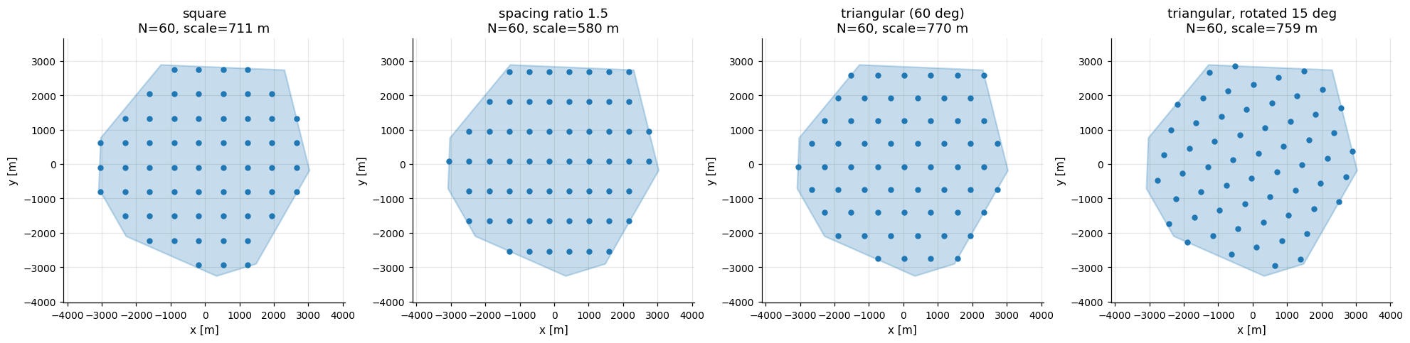
Grid fills a lattice of two grid vectors. spacing_ratio is the length of the second relative to the first, lattice_angle the angle between them and rotation the direction of the first. The defaults give a square lattice. Ratio 1 with a 60° angle gives a triangular one.

grid_shape = B.RandomRadialPolygon(area=np.pi * 3000**2, seed=7)
grid_configs = {
    "square": dict(),
    "spacing ratio 1.5": dict(spacing_ratio=1.5),
    "triangular (60 deg)": dict(lattice_angle=60),
    "triangular, rotated 15 deg": dict(lattice_angle=60, rotation=15),
}

fig, axes = plt.subplots(1, 4, figsize=(18, 4.5))
for ax, (label, kwargs) in zip(axes, grid_configs.items()):
    farm = oowl.Sampler(grid_shape, L.Grid(60, seed=42, **kwargs)).sample()[0]
    farm.plot(
        ax=ax,
        title=f"{label}\nN={farm.n_turbines}, scale={farm.metadata['fit']['scale']:.0f} m",
    )
fig.tight_layout()

Circular

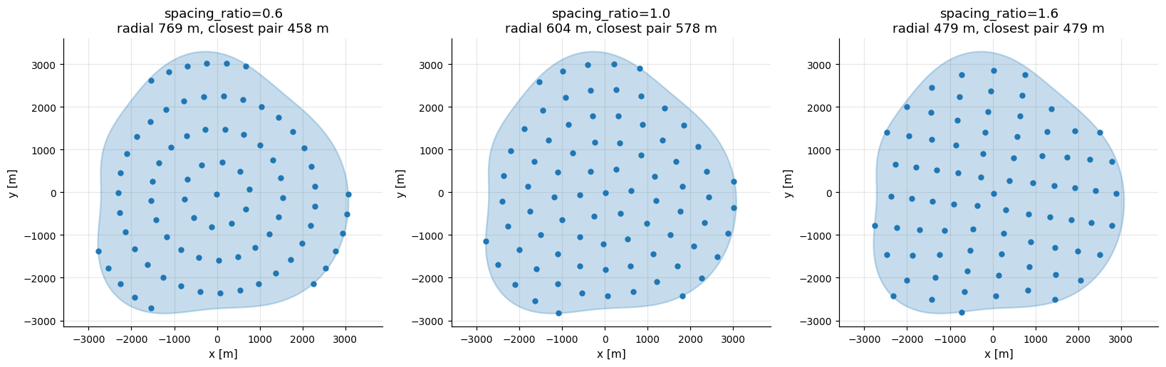
Circular fills concentric rings around the boundary centroid, or around an interior point when the centroid falls outside. spacing_ratio is the spacing along a ring over the radial spacing.

fig, axes = plt.subplots(1, 3, figsize=(15, 4.8))
for ax, ratio in zip(axes, (0.6, 1.0, 1.6)):
    farm = oowl.Sampler(boundary, L.Circular(80, seed=4, spacing_ratio=ratio)).sample()[
        0
    ]
    farm.plot(
        ax=ax,
        title=(
            f"spacing_ratio={ratio}\nradial {farm.metadata['fit']['scale']:.0f} m,"
            f" closest pair {farm.minimum_spacing():.0f} m"
        ),
    )
fig.tight_layout()

Contour

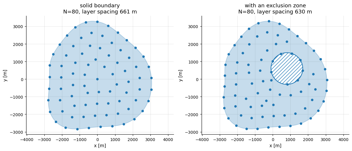
Contour spaces turbines by arc length along repeated inward offsets of the boundary, plus one central point. A hole gets its own contour lines.

holed = boundary.modify(
    M.ExclusionZones([B.Circle(area=np.pi * 900**2, center=(800, 600))])
)

fig, axes = plt.subplots(1, 2, figsize=(11, 4.8))
for ax, (label, boundary) in zip(
    axes, {"solid boundary": boundary, "with an exclusion zone": holed}.items()
):
    farm = oowl.Sampler(boundary, L.Contour(80, seed=4)).sample()[0]
    farm.plot(
        ax=ax,
        title=f"{label}\nN={farm.n_turbines}, layer spacing"
        f" {farm.metadata['fit']['scale']:.0f} m",
    )
fig.tight_layout()

Sunflower

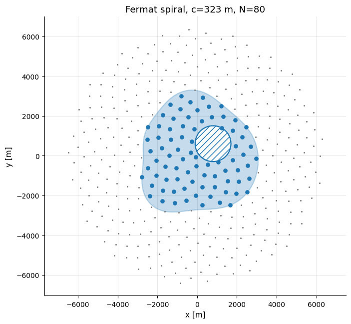
Sunflower places candidates on the Fermat spiral \(r_i = c\sqrt{i}\), \(\theta_i = i\gamma + \theta_0\) of Vogel (1979), with golden angle \(\gamma = \pi(3-\sqrt5)\), centered on the boundary centroid, or on an interior point when the centroid falls outside. The center always holds a turbine. Only contained candidates are kept, \(c\) is the largest value that leaves at least \(N\) of them, and an exact, well-spread subset of \(N\) is selected. The recorded scale is that \(c\).

sunflower = oowl.Sampler(boundary, L.Sunflower(80, seed=4)).sample()[0]
fit = sunflower.metadata["fit"]
index = np.arange(400)
angle = index * np.deg2rad(fit["golden_angle_degrees"]) + np.deg2rad(fit["rotation"])
radius = fit["scale"] * np.sqrt(index)
spiral = np.array(fit["origin"]) + np.column_stack(
    [radius * np.cos(angle), radius * np.sin(angle)]
)

fig, ax = plt.subplots(figsize=(6.5, 6))
sunflower.plot(
    ax=ax,
    s=22,
    title=f"Fermat spiral, c={fit['scale']:.0f} m, N={sunflower.n_turbines}",
)
ax.plot(spiral[:, 0], spiral[:, 1], ".", ms=2, color="C7", zorder=1)
fig.tight_layout()

Scattered families

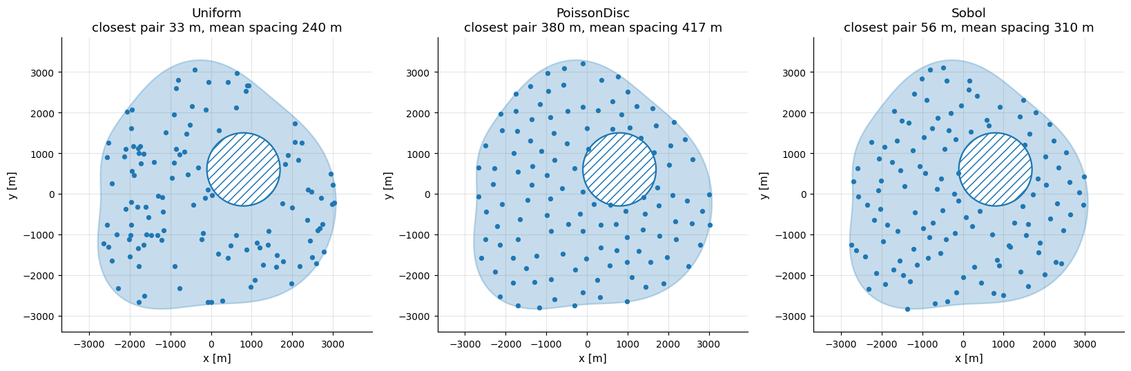
These place turbines without a lattice and differ in what they impose on the scatter. Each farm records its fit in metadata["fit"].

scattered = {
    "Uniform": L.Uniform(120, seed=42),
    "PoissonDisc": L.PoissonDisc(120, seed=42),
    "Sobol": L.Sobol(120, seed=42),
}

fig, axes = plt.subplots(1, 3, figsize=(15, 5))
for ax, (name, layout) in zip(axes, scattered.items()):
    farm = oowl.Sampler(boundary, layout).sample()[0]
    farm.plot(
        ax=ax,
        s=14,
        title=(
            f"{name}\nclosest pair {farm.minimum_spacing():.0f} m,"
            f" mean spacing {farm.mean_spacing():.0f} m"
        ),
    )
    print(f"{name:12s} {farm.metadata['fit']}")
fig.tight_layout()

Uniform      {'method': 'uniform'}
PoissonDisc  {'method': 'poisson_disc', 'scale': 6155.038624499591, 'translation': [-57.66894182964848, 4.374087804586965], 'minimum_distance': 0.06072689121615714, 'k': 30}
Sobol        {'method': 'sobol', 'scramble_seed': 351999658, 'sequence_size': 256, 'accepted_candidates': 185}

Uniform

Uniform is complete spatial randomness. It splits the boundary into triangles, picks one by area and draws a uniform point inside it, so pairs may fall arbitrarily close. It is the null model for Spatial metrics. The wind direction model oowl.resources.UniformDirection is unrelated.

Poisson disc

PoissonDisc seeks blue noise with minimum distance \(d\) by Bridson’s active-list method. Each active point proposes up to k points between radii \(d\) and \(2d\) and retires when none lies inside and at least \(d\) from all others. \(d\) shrinks until at least \(N\) samples exist, and farthest-point subsampling cuts a surplus to \(N\). See Robert Bridson, “Fast Poisson Disk Sampling in Arbitrary Dimensions” (SIGGRAPH 2007).

Sobol

Sobol covers space more evenly than chance with a scrambled, balanced power-of-two sequence over the bounding box. It returns the first \(N\) points inside, raising the power if short, and guarantees no minimum gap.

Boundary-conforming families

These work in realized coordinates and follow concave shapes.

Boundary grid

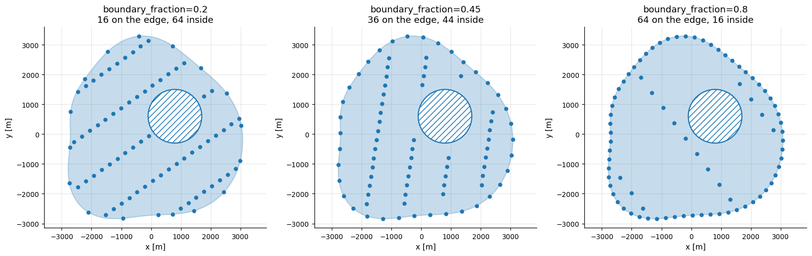
BoundaryGrid spaces up to boundary_fraction of the turbines around the exterior and fills the rest with a centered, rotated inner grid, recorded as boundary_count and grid_count. It is the generator from Stanley and Ning, “Massive simplification of the wind farm layout optimization problem”, Wind Energy Science 4 (2019), 663 to 676, without the optimization.

fig, axes = plt.subplots(1, 3, figsize=(15, 4.8))
for ax, fraction in zip(axes, (0.2, 0.45, 0.8)):
    farm = oowl.Sampler(
        boundary, L.BoundaryGrid(80, seed=4, boundary_fraction=fraction)
    ).sample()[0]
    fit = farm.metadata["fit"]
    farm.plot(
        ax=ax,
        title=(
            f"boundary_fraction={fraction}\n{fit['boundary_count']} on the edge,"
            f" {fit['grid_count']} inside"
        ),
    )
fig.tight_layout()

Perimeter

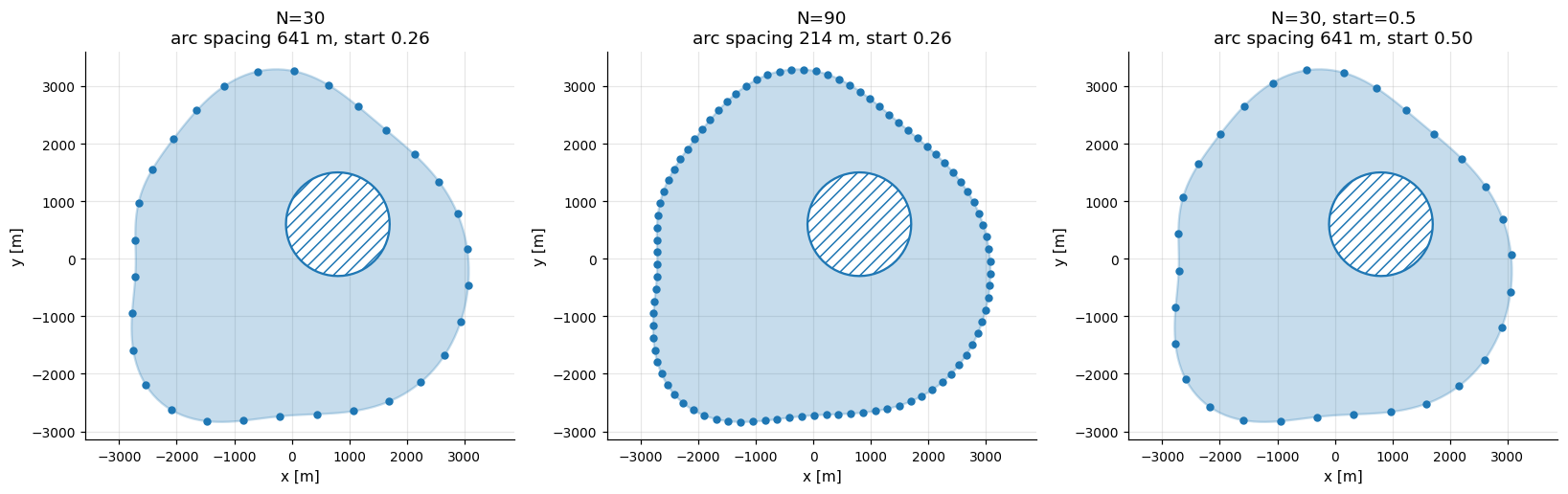
Perimeter spaces every turbine by arc length along the exterior from a start fraction in \([0, 1)\), drawn from the seed when omitted. The spacing is perimeter length over \(N\), recorded as arc_spacing. start rotates the positions without changing it.

perimeter_configs = {
    "N=30": dict(n_turbines=30),
    "N=90": dict(n_turbines=90),
    "N=30, start=0.5": dict(n_turbines=30, start=0.5),
}

fig, axes = plt.subplots(1, 3, figsize=(15, 4.8))
for ax, (label, kwargs) in zip(axes, perimeter_configs.items()):
    farm = oowl.Sampler(boundary, L.Perimeter(seed=4, **kwargs)).sample()[0]
    fit = farm.metadata["fit"]
    farm.plot(
        ax=ax,
        title=f"{label}\narc spacing {fit['arc_spacing']:.0f} m,"
        f" start {fit['start']:.2f}",
    )
fig.tight_layout()

Delaunay

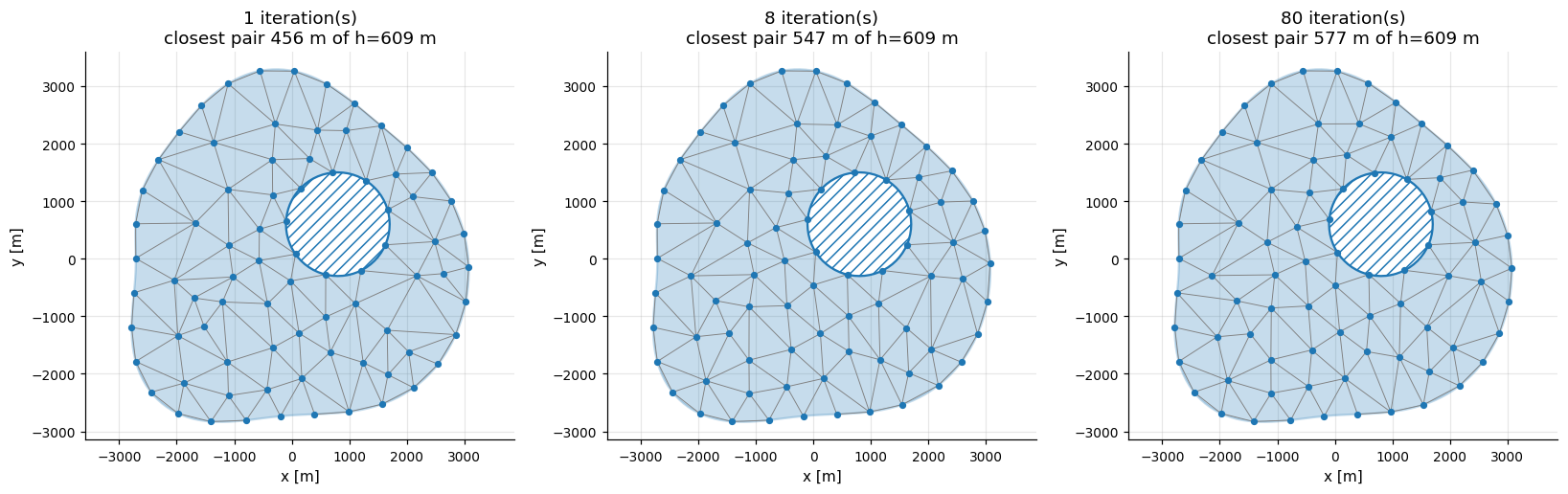
Delaunay spaces nodes evenly along the exterior and hole rings, fills the interior and relaxes all of them toward an even triangular mesh, the edge nodes sliding along their ring. The number of edge nodes follows from the equilateral spacing

\[ h=\sqrt{\frac{2A}{\sqrt3N}}. \]

Each iteration pushes apart the two nodes of every Delaunay edge shorter than \(0.95h\), so nodes either side of a narrow notch keep apart and the settled closest pair lies near \(0.95h\). The relaxation is adapted from Persson and Strang, “A Simple Mesh Generator in MATLAB”, SIAM Review 46 (2004), 329 to 345, with a fixed edge length and the adaptive restart of O’Donoghue and Candès, “Adaptive Restart for Accelerated Gradient Schemes”, Foundations of Computational Mathematics 15 (2015), 715 to 732. The triangles and edges are kept in the metadata.

fig, axes = plt.subplots(1, 3, figsize=(15, 4.8))
for ax, iterations in zip(axes, (1, 8, 80)):
    farm = oowl.Sampler(
        boundary, L.Delaunay(80, seed=4, max_iterations=iterations)
    ).sample()[0]
    fit = farm.metadata["fit"]
    farm.plot(
        ax=ax,
        s=14,
        title=(
            f"{iterations} iteration(s)\nclosest pair {farm.minimum_spacing():.0f} m"
            f" of h={fit['target_spacing']:.0f} m"
        ),
    )
    ax.triplot(farm.x, farm.y, fit["triangles"], color="C7", lw=0.6, zorder=1)
fig.tight_layout()

Related pages are Fitting a pattern to a boundary, Combining layout families, Multipart boundaries and clusters, Layout modifiers, Spatial metrics, Describing a population of farms, Sampling with a density and Drawing, streaming and replaying a population.