Fitted offshore models

FourierPolygon and OffshorePolygon are learned from real offshore wind-farm geometry. They describe a population, not named farms, so the only meaningful comparison with the references is distributional.

Both were fitted to the EMODnet Human Activities wind-farm polygons (CC BY 4.0), as curated in Offshore reference farms and reconciled with EuroWindWakes turbine records. The cohort is 89 operating, fixed-bottom, single-project polygons with at least five turbines. Groups, concept zones, linear farms, demonstrations, floating farms and multipart boundaries are excluded.

Each polygon is repaired if necessary, oriented counterclockwise and simplified with the tolerance

\[ \varepsilon = 0.002\sqrt{A}, \]

for area \(A\) in square meters, then centered and scaled to unit area. Alignment also removes rotation and ring starting point. Both models therefore describe shape alone, whatever the position, rotation or area of a farm, and the requested center and area are applied after sampling. Both share area, center and rotation with the shapes in Boundary shapes.

import matplotlib.pyplot as plt

from oowl import boundaries as B

FourierPolygon

The simplified exterior is resampled at 512 equal-arclength positions as a complex closed curve

\[z_j = x_j + i y_j, \qquad j = 0,\ldots,511.\]

Generalized Procrustes alignment fixes cyclic start, rotation and reflection. The real and imaginary parts of \(Z=\operatorname{FFT}(z)\) form one real vector. PCA retaining 95% of the variance needs nine components, with a Ledoit-Wolf shrinkage score covariance \(\Sigma_s\). For a standard-normal draw \(u\),

\[ s = \tau L u, \qquad Z^{*} = \bar Z + sP, \qquad z^{*} = \operatorname{IFFT}(Z^{*}), \]

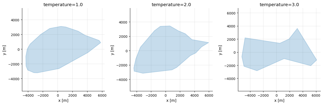
where \(P\) holds the PCA loadings and \(L\) is calibrated so that temperature \(\tau = 2\) reproduces \(\Sigma_s\). Other values narrow or widen the population by scaling every mode together. Scores are correlated across frequencies, and \(Z_0\) is zero to keep the centering. The curve is then simplified toward a vertex count from a shifted-lognormal model, \(\log(V-2)\sim\mathcal N(\mu_V,\sigma_V^2)\), and invalid samples are rejected.

The representation follows Kuhl and Giardina, “Elliptic Fourier features of a closed contour”, Computer Graphics and Image Processing 18 (1982), 236-258. The Gaussian score distribution is a generative assumption, not a claim about real leases.

fig, axes = plt.subplots(1, 3, figsize=(12, 4.0))
for ax, temperature in zip(axes, (1.0, 2.0, 3.0)):
    boundary = B.FourierPolygon(area=40e6, temperature=temperature, seed=20)
    boundary.plot(ax=ax, title=f"temperature={temperature}")
fig.tight_layout()

OffshorePolygon

OffshorePolygon separates global lease shape from local concavity. For 64 directions \(\theta_k\) the convex hull is represented by its support function

\[ h(\theta_k)=\max_{x\in P} x\cdot(\cos\theta_k,\sin\theta_k). \]

After cyclic and reflection alignment, a 99%-variance PCA models the support values with 12 components. Intersecting the half-planes \(x\cdot n_k\le h(\theta_k)\) gives a valid convex envelope. Its corner count is sampled independently from a fitted shifted-lognormal model, and the envelope is simplified to that count with Douglas-Peucker. Every convex shape holds a polygon of \(k\) corners covering at least \(\tfrac{k}{2\pi}\sin\tfrac{2\pi}{k}\) of its area, 0.41 for a triangle, so a simplification that keeps less is redone by dropping, one by one, the corners that cost the least area.

Each non-convex path between consecutive hull corners is mapped to local coordinates with endpoints \((0,0)\) and \((1,0)\) and resampled to 22 landmarks. Four PCA components retain 95.97% of the path shape variance. Their scores, log indentation area and log corner count are sampled jointly from a posterior-predictive multivariate distribution. For an envelope with \(m\) edges,

\[p\sim\operatorname{Beta}(\alpha,\beta),\qquad K\mid p\sim\operatorname{Binomial}(m,p),\]

and the \(K\) irregular edges are drawn without replacement in proportion to edge length. Paths are placed on those edges pointing inward. The model stores only PCA parameters and distributions, never reference polygons.

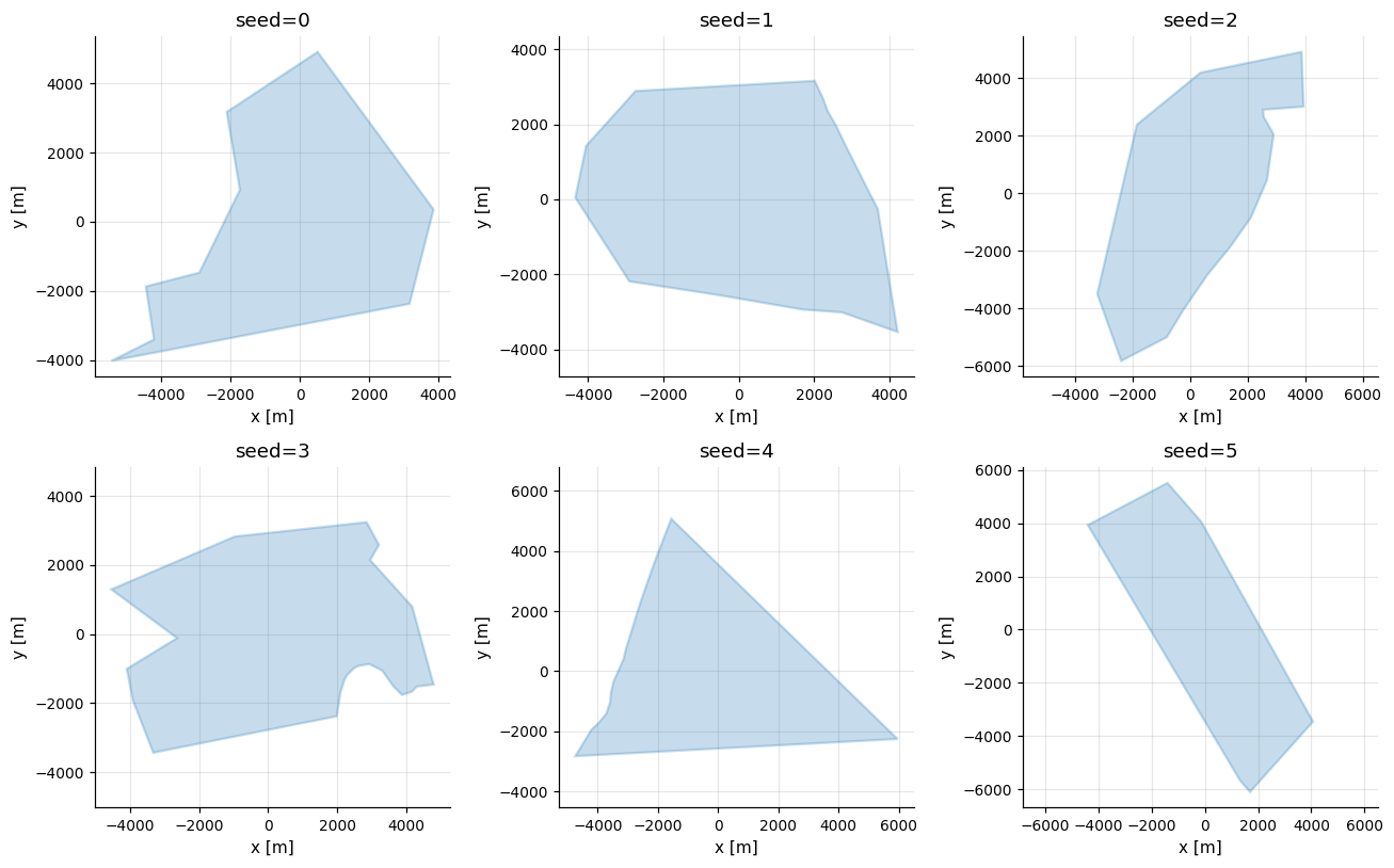
fig, axes = plt.subplots(2, 3, figsize=(12, 7.5))
for ax, seed in zip(axes.flat, range(6)):
    boundary = B.OffshorePolygon(area=40e6, seed=seed)
    boundary.plot(ax=ax, title=f"seed={seed}")
fig.tight_layout()

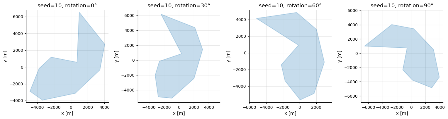
Alignment discarded each training heading, so a sample draws one uniformly. With a fixed seed, rotation turns the same shape to a heading in degrees counterclockwise about its centroid.

fig, axes = plt.subplots(1, 4, figsize=(14, 3.8))
for ax, heading in zip(axes, (0, 30, 60, 90)):
    boundary = B.OffshorePolygon(area=40e6, rotation=heading, seed=10)
    boundary.plot(ax=ax, title=f"seed=10, rotation={heading}°")
fig.tight_layout()

Differences and limitations

Property	FourierPolygon	OffshorePolygon
Global representation	512-point closed curve	64-direction convex support function
Local non-convexity	Implicit in global Fourier modes	Explicit normalized edge paths
Retained dimensions	9 global components	12 envelope + 4 path components
Vertex complexity	One exterior-count model	Separate hull and edge-path counts
Distribution control	temperature, fitted value is 2	Fixed fitted population
Interpretation	Frequency-domain curve variation	Envelope, irregular-edge occupancy, indentation shape and area

Both models were refitted in five geographically grouped outer folds. Held-out polygons were compared with generated ensembles on compactness, convexity, rectangularity, elongation, roughness and standardized vertex complexity. A classifier AUC near 0.5 means these descriptors barely distinguish real from generated polygons.

Diagnostic	FourierPolygon	OffshorePolygon
Normalized Wasserstein, mean	0.276	0.218
Linear classifier AUC	0.657	0.529
Random-forest classifier AUC	0.710	0.558
Held-out values inside generated 90% intervals	82.4%	86.9%
Valid and unique stress samples	5,000 / 5,000	10,000 / 10,000
Exact reference copies	0	0

The runs used different repeat counts, so this is not a formal significance test. OffshorePolygon matches better, but its random-forest AUC narrowly misses the target of 0.55. OOWL does not claim that generated and real boundaries are indistinguishable.

The population covers operating European fixed-bottom projects in the source snapshot. It does not describe floating leases, linear farms, multipart projects, future planning zones or trends in lease policy. Area is supplied independently, so neither model captures dependence between area and shape, and neither conditions on turbine count, era, country or layout.