Boundary shapes

A boundary is the admissible region of a wind-farm study, used by layout generation and boundary-aware metrics. It wraps a valid Shapely Polygon or MultiPolygon in meters.

A constructor builds an unscaled geometry \(G\) of area \(A_G\). A target area \(A\) applies the isotropic factor

\[ s = \sqrt{\frac{A}{A_G}} \]

about the centroid of \(G\), which is then moved to center. Dimensions set proportions and area sets size. Polygon keeps its coordinates unless area or center is given. Every boundary must be valid with positive area.

Fitted offshore models are in Fitted offshore models. Exclusions, setbacks and partitions are in Boundary modifiers.

import matplotlib.pyplot as plt
import numpy as np
import shapely

from oowl import boundaries as B


def show(boundaries, figsize=(12, 3.6)):
    """Plot one row of named boundaries, each titled with its own area."""
    fig, axes = plt.subplots(1, len(boundaries), figsize=figsize)
    for ax, (name, boundary) in zip(axes, boundaries.items()):
        boundary.plot(ax=ax, title=f"{name}\n{boundary.area / 1e6:.1f} km²")
    fig.tight_layout()

Primitive shapes

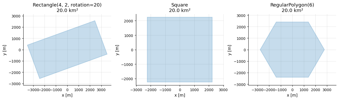
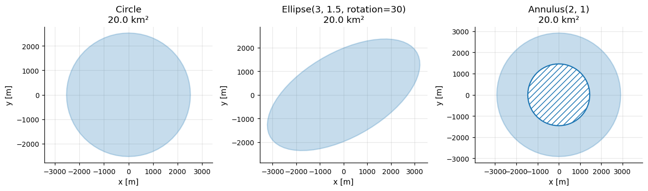
Primitives share area, center and, where meaningful, rotation in degrees counterclockwise. Rectangle width and height, Ellipse semi-axes and Annulus radii fix only proportions. Curved primitives are polygons with n_segments vertices, worth raising for perimeter-sensitive metrics. The annulus hole is part of the shape, not an exclusion.

show(
    {
        "Rectangle(4, 2, rotation=20)": B.Rectangle(4, 2, area=20e6, rotation=20),
        "Square": B.Square(area=20e6),
        "RegularPolygon(6)": B.RegularPolygon(6, area=20e6),
    }
)
show(
    {
        "Circle": B.Circle(area=20e6),
        "Ellipse(3, 1.5, rotation=30)": B.Ellipse(3, 1.5, area=20e6, rotation=30),
        "Annulus(2, 1)": B.Annulus(2, 1, area=20e6),
    }
)

Radial shapes

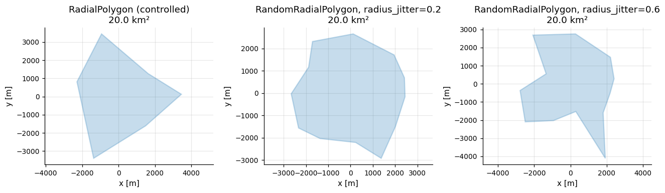
Both radial families are star-shaped about the origin they are generated around. RadialPolygon takes one radius and one positive angular step in degrees per vertex,

\[ x_i = r_i\cos\theta_i, \qquad y_i = r_i\sin\theta_i, \]

where \(\theta_i\) is the cumulative sum of the steps converted to radians. The shape is then scaled to its area and its centroid placed at center, which need not be the origin. RandomRadialPolygon perturbs both around a regular polygon by radius_jitter and angular_jitter, renormalizing the steps to sum to \(2\pi\) and keeping radii positive.

radii = [1.0, 2.0, 1.5, 2.2, 1.2, 1.8]
angular_offsets = [40, 70, 55, 80, 60, 55]
radial = {
    "RadialPolygon (controlled)": B.RadialPolygon(radii, angular_offsets, area=20e6),
    "RandomRadialPolygon, radius_jitter=0.2": B.RandomRadialPolygon(
        12, area=20e6, radius_jitter=0.2, seed=3
    ),
    "RandomRadialPolygon, radius_jitter=0.6": B.RandomRadialPolygon(
        12, area=20e6, radius_jitter=0.6, seed=3
    ),
}
show(radial)

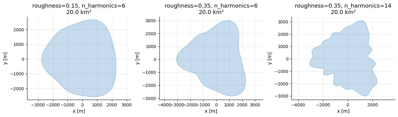
SmoothBlob uses the random radius function

\[ r(\theta) = 1 + \sum_{k=1}^{K}\frac{\rho\,\xi_k}{k}\sin(k\theta + \phi_k), \]

with standard-normal \(\xi_k\), uniform phases \(\phi_k\) and roughness \(\rho\). The radius is clipped away from zero. Raising n_harmonics adds finer structure, and raising n_segments only samples the same curve more densely.

blobs = {
    f"roughness={roughness}, n_harmonics={n_harmonics}": B.SmoothBlob(
        area=20e6, roughness=roughness, n_harmonics=n_harmonics, seed=2
    )
    for roughness, n_harmonics in ((0.15, 6), (0.35, 6), (0.35, 14))
}
show(blobs)

Boundaries from data

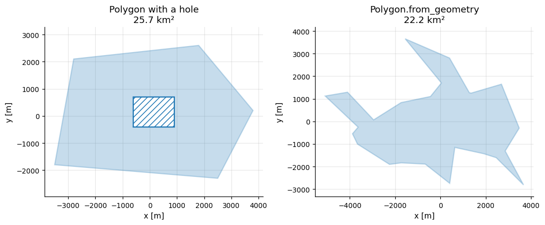
Polygon accepts vertices and holes, and Polygon.from_geometry accepts a Shapely Polygon or MultiPolygon, here the concave hull of a measured point cloud. Interior rings are excluded from layouts. Coordinates are kept as given unless area or center is passed.

OOWL does not repair invalid polygons, since repair can drop rings, split components or change area. Check imported geometry and its coordinate reference system first.

survey = B.Polygon(
    [[-3500, -1800], [2500, -2300], [3800, 200], [1800, 2600], [-2800, 2100]],
    holes=[[[-600, -400], [900, -400], [900, 700], [-600, 700]]],
)
measured = np.random.default_rng(3).normal(scale=[1800.0, 1100.0], size=(60, 2))
imported = B.Polygon.from_geometry(
    shapely.concave_hull(shapely.MultiPoint(measured), ratio=0.4)
)
show({"Polygon with a hole": survey, "Polygon.from_geometry": imported}, (10, 4.2))

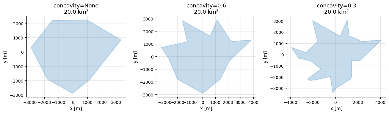
ConvexHull wraps a random point cloud. The default concavity=None gives the exact convex hull. A float in \((0, 1]\) is passed to shapely.concave_hull as its ratio, where 1 is convex and smaller values follow the points more closely. Keep the ratio high, because small ratios follow sampling density. For realistic lease outlines use Fitted offshore models.

show(
    {
        f"concavity={concavity}": B.ConvexHull(
            n_points=40, area=20e6, concavity=concavity, seed=5
        )
        for concavity in (None, 0.6, 0.3)
    }
)

Unions

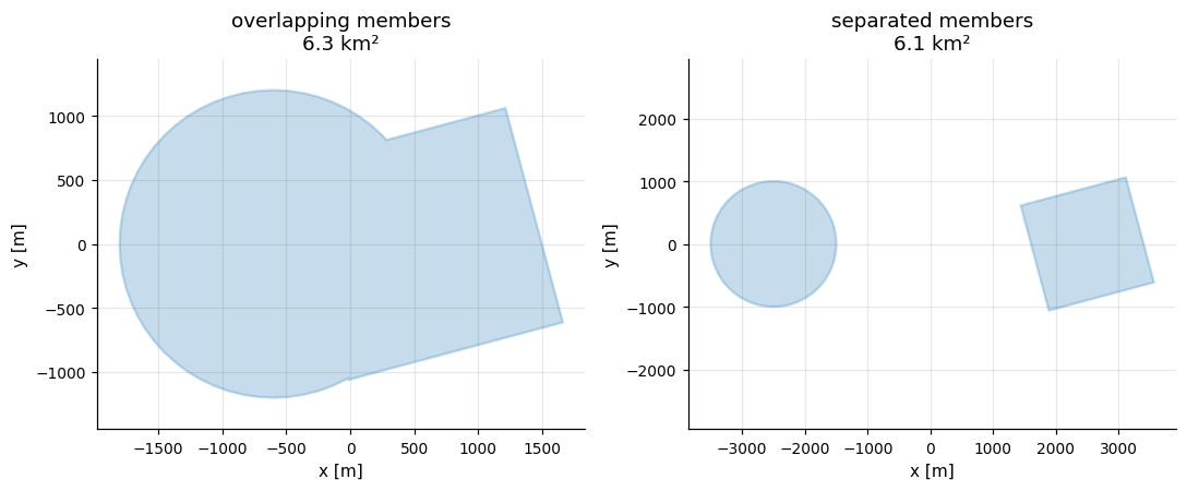
Union merges overlapping members into one polygon and keeps separated members as one multipart boundary. The result is one farm. Each member keeps its own size, and area on the Union sets the area of the combined result.

show(
    {
        "overlapping members": B.Union(
            [
                B.Circle(area=np.pi * 1200**2, center=(-600, 0)),
                B.Square(area=3e6, center=(600, 0), rotation=15),
            ]
        ),
        "separated members": B.Union(
            [
                B.Circle(area=np.pi * 1000**2, center=(-2500, 0)),
                B.Square(area=3e6, center=(2500, 0), rotation=15),
            ]
        ),
    },
    (10, 4.2),
)