Layout optimization with TOPFARM

TOPFARM moves turbines to maximize energy yield within a boundary and a minimum spacing. OOWL supplies the starting layout and boundary, and PyWake from Energy yield with PyWake supplies the objective.

TOPFARM is not an OOWL dependency.

%%capture
%pip install --quiet topfarm

Import OOWL, PyWake and TOPFARM.

import contextlib
import io

import matplotlib.pyplot as plt
import numpy as np
import shapely
import xarray as xr
from py_wake.literature.gaussian_models import Bastankhah_PorteAgel_2014
from py_wake.site import XRSite
from py_wake.wind_turbines import WindTurbine
from py_wake.wind_turbines.power_ct_functions import PowerCtTabular
from topfarm import TopFarmProblem
from topfarm.constraint_components.boundary import XYBoundaryConstraint
from topfarm.constraint_components.spacing import SpacingConstraint
from topfarm.cost_models.py_wake_wrapper import PyWakeAEPCostModelComponent
from topfarm.easy_drivers import EasyScipyOptimizeDriver

import oowl
from oowl import boundaries as B
from oowl import layouts as L
from oowl import resources as R
from oowl import turbines as T

/builds/sys/OOWL/.pixi/envs/dev/lib/python3.12/site-packages/pyDOE2/doe_factorial.py:201: SyntaxWarning: invalid escape sequence '\-'
  A = [item for item in re.split('\-|\s|\+', gen) if item]  # remove empty strings

The starting layout

The boundary, Sunflower layout and resource match Energy yield with PyWake, with identical parameters and seeds.

boundary = B.RandomRadialPolygon(
    n_vertices=7, area=36e6, radius_jitter=0.4, angular_jitter=0.4, seed=16
)
turbine = T.Idealized(
    rated_power=15e6, rotor_diameter=240.0, hub_height=150.0, cp_max=0.48
)
resource = R.WindResource(
    direction=R.VonMises(n_modes=1, seed=3),
    n_sectors=12,
    mean_wind_speed=9.5,
    weibull_k=2.2,
    turbulence=R.SurfaceLayer(intensity=0.07),
    reference_height=turbine.hub_height,
)
farm = oowl.Sampler(
    boundary,
    L.Sunflower(n_turbines=16, seed=5),
    resource,
    turbines=turbine,
    seed=4,
).sample()[0]

The turbine and resource map to PyWake as in Energy yield with PyWake. The AEP of the starting layout is the reference for the optimized layout.

speeds = np.arange(0.0, 30.5, 0.5)
wind_turbine = WindTurbine(
    name="OOWL idealized 15 MW",
    diameter=turbine.rotor_diameter,
    hub_height=turbine.hub_height,
    powerCtFunction=PowerCtTabular(
        speeds, turbine.power(speeds), "W", turbine.ct(speeds)
    ),
)
site = XRSite(
    xr.Dataset(
        data_vars={
            "Sector_frequency": ("wd", resource.probability),
            "Weibull_A": ("wd", resource.weibull_a),
            "Weibull_k": ("wd", resource.weibull_k),
            "TI": ("wd", resource.sector_turbulence_intensity),
        },
        coords={"wd": resource.theta},
    )
)
wfm = Bastankhah_PorteAgel_2014(site, wind_turbine, k=0.0324555)

simulation = wfm(farm.x, farm.y)
net = float(simulation.aep().sum())
gross = float(simulation.aep(with_wake_loss=False).sum())
print(f"starting layout gross {gross:.1f} GWh, net {net:.1f} GWh")

starting layout gross 1258.5 GWh, net 1186.9 GWh

OOWL boundary → TOPFARM constraints

The boundary exterior becomes an XYBoundaryConstraint of type "polygon", since "convex_hull" would give the optimizer the notch of this non-convex boundary. SpacingConstraint takes meters, here three rotor diameters, which the starting layout already satisfies.

vertices = np.asarray(boundary.geometry.exterior.coords)[:-1]
constraints = [
    XYBoundaryConstraint(vertices, "polygon"),
    SpacingConstraint(3 * turbine.rotor_diameter),
]
print(f"TOPFARM constraints prepared for {len(vertices)} boundary vertices")

TOPFARM constraints prepared for 7 boundary vertices

PyWakeAEPCostModelComponent makes PyWake the objective and SLSQP moves the turbines. Iterations are capped for build time. A real study should run to convergence from several starting layouts.

problem = TopFarmProblem(
    design_vars={"x": farm.x, "y": farm.y},
    cost_comp=PyWakeAEPCostModelComponent(wfm, n_wt=farm.n_turbines),
    constraints=constraints,
    driver=EasyScipyOptimizeDriver(optimizer="SLSQP", maxiter=120, disp=False),
    expected_cost=1e-2,
)
# Suppress SLSQP's capped-iteration termination output.
with contextlib.redirect_stdout(io.StringIO()):
    _, state, _ = problem.optimize(disp=False)
optimized_farm = oowl.Farm(
    positions=np.column_stack([state["x"], state["y"]]),
    boundary=boundary,
    resource=resource,
    turbines=farm.turbines,
)

Optimized layout

Compare the optimized positions and AEP with the starting layout.

optimized = float(wfm(optimized_farm.x, optimized_farm.y).aep().sum())
print(f"AEP {net:.1f} -> {optimized:.1f} GWh ({100 * (optimized / net - 1):+.2f} %)")
print(
    f"wake loss {100 * (1 - net / gross):.2f} % -> {100 * (1 - optimized / gross):.2f} %"
)

fig, axes = plt.subplots(1, 2, figsize=(11, 4), constrained_layout=True)
panels = (
    (farm, f"OOWL starting layout, {net:.0f} GWh"),
    (optimized_farm, f"TOPFARM optimized, {optimized:.0f} GWh"),
)
for ax, (drawn, title) in zip(axes, panels):
    drawn.plot(ax=ax, title=title)

AEP 1186.9 -> 1221.5 GWh (+2.91 %)
wake loss 5.69 % -> 2.94 %

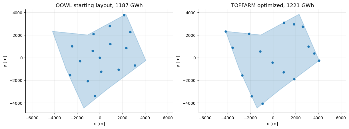
The optimizer moves turbines out to the boundary and recovers part of the wake loss. The boundary check measures distance, since SLSQP meets the boundary constraint only to within its tolerance.

excursion = shapely.distance(
    shapely.points(optimized_farm.positions), boundary.geometry
).max()
print(f"furthest any turbine sits outside the boundary: {excursion:.3g} m")

print(f"starting closest pair {farm.minimum_spacing():.1f} m")
for name, drawn in (("starting", farm), ("optimized", optimized_farm)):
    summary = drawn.summary()
    print(
        f"{name:>9}: mean spacing {summary['nearest_neighbor_mean']:7.1f} m,"
        f" variation {summary['nearest_neighbor_variation']:.3f}"
    )

furthest any turbine sits outside the boundary: 1.97e-08 m
starting closest pair 881.4 m
 starting: mean spacing  1396.4 m, variation 0.148
optimized: mean spacing  1195.4 m, variation 0.325

Next steps

Cable routing with OptiWindNet connects the farm to a substation, and Layout families explores other starting layouts.