Coverage design

R.Dimitrov draws training cases for a surrogate that must hold at any site (Dimitrov et al., 2018). The cases spread evenly between bounds that hold nearly all site conditions, so the surrogate seldom extrapolates, and the checks below show what falls outside. They are not weighted by how often they occur, so the energy, loads and statistics of a real site come from a resource of Wind resources. A rotor diameter adds the veer across the rotor.

import matplotlib.pyplot as plt
import numpy as np
from matplotlib.colors import LogNorm
from scipy import stats

import oowl
from oowl import resources as R

height = 100.0
design = R.Dimitrov(reference_height=height)
cases = design.sample(8192, seed=1)
print(design)

Dimitrov(minimum_intensity=0.025, reference_intensity=0.18, maximum_intensity=None, roughness_range=(1e-05, 1), heat_flux=0.3, temperature_scale=0.3, rotor_diameter=None, latitude=50, n_sectors=12, reference_height=100)

A recipe draws one design per reference height. An argument named *_range keeps its pair, so every design here spans roughness from \(10^{-5}\) to 2 m.

designs = oowl.Sampler(
    resource=(
        R.Dimitrov,
        {"reference_height": (80.0, 150.0), "roughness_range": (1e-5, 2.0)},
    ),
    seed=2,
).sample(3)
print([round(design.reference_height, 1) for design in designs])

[147.2, 118.0, 145.5]

Bounds

Variable	Lower bound	Upper bound	Parameter
\(\sigma_u\)	\(0.025\,U\)	\(0.18\left[6.8 + 0.75U + 3(10/U)^2\right]\)	minimum_intensity, reference_intensity, maximum_intensity
\(z/L\)	\(-z\kappa g H_{\max}/(T_0 u_*^3)\)	\(z\kappa g\theta_{*\max}/(T_0 u_*^2)\)	heat_flux, temperature_scale
\(z_0\)	\(10^{-5}\) m	1 m	roughness_range
Mann \(L\)	\(\max\{7.5\ \mathrm{m}, (15\ \mathrm{m})\,\lvert\alpha\rvert^{-2/3}\}\)	275 m
Mann \(\Gamma\)	1	5
veer	\(-0.1\,D\,(5/U)\)	\(\min\{60^\circ\sin\lvert\phi\rvert, D\,(5/U)^2\}\)	rotor_diameter, latitude
yaw, tilt	\(-10^\circ\)	\(10^\circ\)
\(\rho\)	1.1 kg m⁻³	1.35 kg m⁻³

\(D\) is the rotor diameter in meters, \(\phi\) the latitude and \(\alpha\) the shear exponent at the reference height. The wind speed is uniform over the sampled range and the direction over the sectors. The stability bounds, not in the paper, use \(H_{\max} = 0.3\) K m/s over \(z_0 = 10^{-5}\) m and \(\theta_{*\max} = 0.3\) K, with \(u_*\) from the stable profile at the bound, and cases are uniform in \(\operatorname{asinh}\left[(z/L)/0.1\right]\). At Høvsøre 0.24 percent of records fall outside. The shear follows from \(z_0\) and \(1/L\) through the log law,

\[U(z) \propto \ln\frac{z}{z_0} - \Psi\!\left(\frac{z}{L}\right) + \Psi\!\left(\frac{z_0}{L}\right).\]

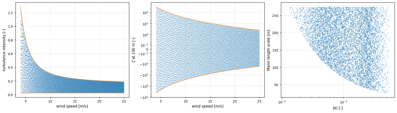
The design at 100 m fills its bounds, and the floor of the Mann length scale rises as shear falls.

u = np.linspace(4.0, 25.0, 200)
sigma_low, sigma_high = design.turbulence.bounds(u)
zeta_low, zeta_high = design.stability.bounds(u, height=height)
style = {"s": 2, "alpha": 0.3}

fig, axes = plt.subplots(1, 3, figsize=(15.0, 4.2), layout="constrained")
axes[0].scatter(cases.wind_speed, cases.turbulence_intensity, **style)
axes[1].scatter(cases.wind_speed, cases.stability_parameter(height), **style)
for ax, (low, high) in zip(
    axes[:2], ((sigma_low / u, sigma_high / u), (zeta_low, zeta_high))
):
    ax.plot(u, low, "C1", lw=1.0)
    ax.plot(u, high, "C1", lw=1.0)
    ax.set_xlabel("wind speed [m/s]")
axes[0].set(ylabel="turbulence intensity [-]")
axes[1].set(ylabel=r"$\zeta$ at 100 m [-]")
axes[1].set_yscale("asinh", linear_width=0.1)
axes[2].scatter(np.abs(cases.shear_exponent), cases.mann_length_scale, **style)
axes[2].set(xscale="log", xlabel=r"$|\alpha|$ [-]", ylabel="Mann length scale [m]");

Veer

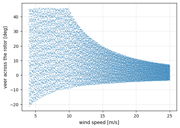
Veer across the rotor scales with its size, so rotor_diameter adds it, here for the DTU 10 MW rotor. The bounds narrow as the wind rises, and in light wind the Coriolis limit at latitude caps the upper one.

rotor = R.Dimitrov(rotor_diameter=178.3, reference_height=height)
veer = rotor.sample(8192, seed=1)
fig, ax = plt.subplots(figsize=(6.0, 4.2))
ax.scatter(veer.wind_speed, veer.wind_veer, **style)
ax.set(xlabel="wind speed [m/s]", ylabel="veer across the rotor [deg]");

Physical sites

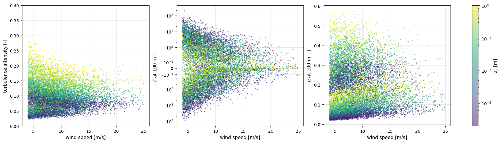
One case from each of 10000 drawn sites shows the conditions real sites produce. The roughness is log-uniform from open water, \(2 \times 10^{-4}\) m, to forest, 1 m, with the mean wind speed, Weibull shape, stability climate and turbulence coefficient ranged per site, see Stability and turbulence. Rougher sites are more turbulent and more sheared. The two bands of shear are unstable air, at about 0.65 times the neutral \(1/\ln(z/z_0)\), and stable air, at about 2.3 times it.

sites = oowl.Sampler(
    resource=(
        R.WindResource,
        {
            "direction": (R.VonMises, {"n_modes": (1, 3)}),
            "mean_wind_speed": (5.0, 11.0),
            "weibull_k": (1.8, 2.6),
            "roughness_length": stats.loguniform(2e-4, 1.0),
            "stability": (
                R.KellyGryning,
                {
                    "unstable_fraction": (0.3, 0.7),
                    "stable_scale": (0.005, 0.02),
                    "unstable_scale": (0.01, 0.035),
                },
            ),
            "turbulence": R.SurfaceLayer(coefficient=stats.uniform(1.8, 0.7)),
        },
    ),
    seed=5,
).sample(10_000)

pooled = [site.sample(1, seed=index) for index, site in enumerate(sites)]
speed = np.concatenate([c.wind_speed for c in pooled])
intensity = np.concatenate([c.turbulence_intensity for c in pooled])
zeta = np.concatenate([c.stability_parameter(100.0) for c in pooled])
shear = np.concatenate([c.shear_exponent for c in pooled])
roughness = np.concatenate([c.roughness_length for c in pooled])

fig, axes = plt.subplots(1, 3, figsize=(15.0, 4.2), layout="constrained")
style = {"c": roughness, "norm": LogNorm(2e-4, 1.0), "s": 2, "alpha": 0.5}
axes[0].scatter(speed, intensity, **style)
axes[1].scatter(speed, zeta, **style)
points = axes[2].scatter(speed, shear, **style)
fig.colorbar(points, ax=axes, label="$z_0$ [m]")
axes[0].set(ylim=(0.0, 0.4), ylabel="turbulence intensity [-]")
axes[1].set(ylabel=r"$\zeta$ at 100 m [-]")
axes[1].set_yscale("asinh", linear_width=0.1)
axes[2].set(ylabel=r"$\alpha$ at 100 m [-]")
for ax in axes:
    ax.set_xlabel("wind speed [m/s]")

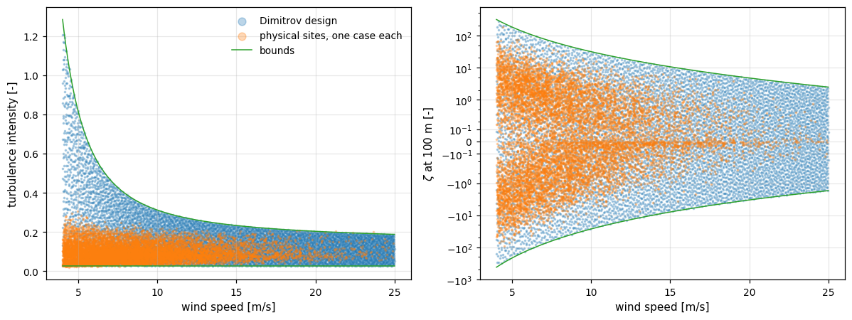
The sites stay within the stability bounds. Their turbulence meets the floor of the band at low wind and its top above about 17 m/s, and a few cases cross them. Below 8 m/s the band top reaches 2 to 4 times the 99th percentile of the sites, where Høvsøre keeps 99.5 percent of records below a TI of 0.23 at 4 to 6 m/s.

style = {"s": 2, "alpha": 0.3}
fig, axes = plt.subplots(1, 2, figsize=(11.0, 4.2))
axes[0].scatter(
    cases.wind_speed, cases.turbulence_intensity, label="Dimitrov design", **style
)
axes[0].scatter(speed, intensity, label="physical sites, one case each", **style)
axes[1].scatter(cases.wind_speed, cases.stability_parameter(height), **style)
axes[1].scatter(speed, zeta, **style)
for ax, (low, high) in zip(
    axes, ((sigma_low / u, sigma_high / u), (zeta_low, zeta_high))
):
    ax.plot(u, low, "C2", lw=1.0)
    ax.plot(u, high, "C2", lw=1.0, label="bounds")
    ax.set_xlabel("wind speed [m/s]")
axes[0].set(ylabel="turbulence intensity [-]")
axes[1].set(ylabel=r"$\zeta$ at 100 m [-]")
axes[1].set_yscale("asinh", linear_width=0.1)
axes[0].legend(markerscale=5, frameon=False)
fig.tight_layout()