Offshore reference farms

OOWL ships a catalog of European fixed-bottom offshore wind farms built from EMODnet boundaries and EuroWindWakes, OpenStreetMap and national agency data. Each farm loads offline as an ordinary Farm and each group as a Cluster.

import matplotlib.pyplot as plt
import numpy as np

import oowl

Load and inspect farms

Names accept aliases, and ambiguous names are refused.

names = ["Horns Rev I", "Anholt", "Moray East"]
fig, axes = plt.subplots(1, 3, figsize=(14, 4.5))
for ax, name in zip(axes, names):
    farm = oowl.reference_farm(name)
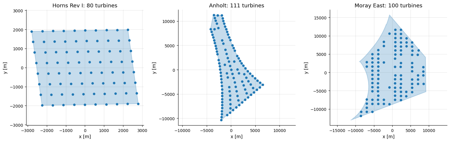
    farm.plot(ax=ax, title=f"{name}: {farm.n_turbines} turbines")
fig.tight_layout()

Sources and citations are kept in metadata.

horns_rev = oowl.reference_farm("Horns Rev I")
print(horns_rev.metadata["boundary_source"])
print(horns_rev.metadata["citations"])

EMODnet
['Fischereit, Vollmer & Hansen, Open European offshore wind turbine database, doi:10.5281/zenodo.19879819', 'OpenStreetMap contributors, current and historical turbine nodes, ODbL 1.0', 'EMODnet Human Activities wind-farm polygons, CC BY 4.0']

Search the catalog

reference_farm.list filters by country, commissioning years and size without loading geometry. Named groups are listed only on request, so no farm appears twice.

danish = oowl.reference_farm.list(country="Denmark")
recent = oowl.reference_farm.list(commissioning_year_range=(2020, 2025))
large = oowl.reference_farm.list(min_turbines=100)
print(f"Danish farms: {len(danish)}")
print(f"Farms commissioned 2020 to 2025: {len(recent)}")
print(f"Farms with at least 100 turbines: {len(large)}, first six")
print([item.name for item in large[:6]])

Danish farms: 17
Farms commissioned 2020 to 2025: 28
Farms with at least 100 turbines: 14, first six
['Anholt', 'East Anglia One', 'Gemini', 'Greater Gabbard', 'Gwynt y Mor', 'Hollandse Kust Zuid']

Project groups and clusters

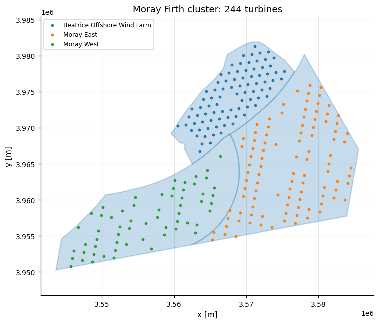
A group such as Borssele Kavel or the Moray Firth cluster loads as a Cluster of its member farms, each with its own boundary and identity.

groups = [
    item for item in oowl.reference_farm.list(include_groups=True) if item.is_group
]
for item in sorted(groups, key=lambda value: value.n_turbines, reverse=True)[:6]:
    print(f"{item.name}: {item.n_turbines} turbines")

group = oowl.reference_farm("Moray Firth cluster", coordinate_frame="epsg:3035")
fig, ax = plt.subplots(figsize=(7, 6))
for index, member in enumerate(group):
    member.plot(ax=ax, s=8, color=f"C{index}", label=member.metadata["name"])
ax.set_title(f"Moray Firth cluster: {group.n_turbines} turbines")
ax.legend(fontsize=8)
fig.tight_layout()

Belgian-Borssele offshore cluster: 571 turbines
Borkum-Gode Wind cluster: 458 turbines
Belgian offshore wind zone: 398 turbines
East Irish Sea cluster: 357 turbines
Hollandse Kust cluster: 348 turbines
German Bight deep-water cluster: 345 turbines

Catalog turbine curves

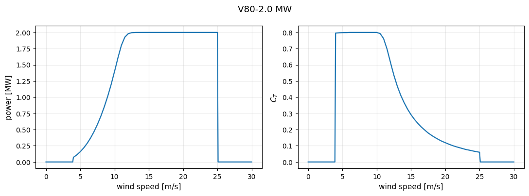
Reference farms carry Tabulated turbines, which interpolate the packaged curves linearly and read zero outside them. Every packaged thrust curve is flat from cut-in to half rated power, with \(C_T\) between 0.796 and 0.800. For a thrust that rises toward cut-in, use a Controlled turbine with the same rating and rotor.

turbine = horns_rev.turbines
speeds = np.linspace(0, 30, 301)
fig, axes = plt.subplots(1, 2, figsize=(10, 3.7))
axes[0].plot(speeds, turbine.power(speeds) / 1e6)
axes[1].plot(speeds, turbine.ct(speeds))
axes[0].set_ylabel("power [MW]")
axes[1].set_ylabel(r"$C_T$")
for ax in axes:
    ax.set_xlabel("wind speed [m/s]")
    ax.grid(alpha=0.25)
fig.suptitle(turbine.name)
fig.tight_layout()

Optional wind resources

oowl.reference_farm("Horns Rev I", resource="gwa") downloads the Global Wind Atlas climate at the farm centroid and caches it on disk. The API reference lists every loading option and catalog field.